1

2


4
Indagate Fingite Invenite (Explore, Dream, Discover)
5
Copyright Statement
This copy of the thesis has been supplied on condition that anyone who consults it is
understood to recognise that its copyright rests with its author and that no quotation
from the thesis and no information derived from it may be published without the
author's prior consent.

6
Author’s declaration
At no time during the registration for the degree of Doctor of Philosophy has the
author been registered for any other University award without prior agreement of the
Doctoral College Quality Sub-Committee. Work submitted for this research degree at
the University of Plymouth has not formed part of any other degree either at University
of Plymouth or at another establishment. This research was financed with the aid of the
Marie Curie Initial Training Network FP7-PEOPLE-2013-ITN-604764.
URL: https://ec.europa.eu/research/mariecurieactions/
Additional information can be found under the following URL:
https://www.cognovo.eu/christopher-germann
E-Mail: mail@christopher.germann.de
Word count of main body of thesis: 71,221
Signed: ___________________________
Date: ___________________________

7
Prefix: Interpretation of the cover illustration
The cover of this thesis depicts a variation of Möbius band which has been
eponymously named after the German astronomer and mathematician August Ferdinand
Möbius. An animated version of the digital artwork and further information can be
found on the following custom-made website:
URL: http://moebius-band.ga
The Möbius band has very peculiar geometrical properties because the inner and the
outer surface create a single continuous surface, that is, it has only one boundary. A
Gedanken-experiment is illustrative: If one imagines walking along the Möbius band
starting from the seam down the middle, one would end back up at the seam, but at the
opposite side. One would thus traverse a single infinite path even though an outside
observer would think that we are following two diverging orbits. We suggest that the
Möbius band can be interpreted as a visual metaphor for dual-aspect monism
(Benovsky, 2016), a theory which postulates that the psychological and the physical are
two aspects of the same penultimate substance, i.e., they are different manifestations of
the same ontology. Gustav Fechner (the founding father of psychophysics) was a
proponent of this Weltanschauung, as were William James, Baruch de Spinoza, Arthur
Schopenhauer, and quantum physicists Wolfgang Pauli and David Bohm, inter alia.
The nondual perspective is incompatible with the reigning paradigm of reductionist
materialism which postulates that matter is ontologically primary and fundamental and
that the mental realm emerges out of the physical, e.g., epiphenomenalism/evolutionary
emergentism (cf. Bawden, 1906; Stephan, 1999)). The nondual perspective has been
concisely articulated by Nobel laureate Bertrand Russel:
“The whole duality of mind and matter [...] is a mistake; there is only one kind of stuff

8
out of which the world is made, and this stuff is called mental in one arrangement,
physical in the other.” (Russell, 1913, p.15)
From a psychophysical perspective it is interesting to note that quantum physicist and
Nobel laureate Wolfgang Pauli and depth psychologist Carl Gustav Jung discussed
dual-aspect monism extensively in their long-lasting correspondence which spanned
many years. In particular, the “Pauli-Jung conjecture” (Atmanspacher, 2012) implies
that psychological and physical states exhibit complementarity in a quantum physical
sense (Atmanspacher, 2014b; Atmanspacher & Fuchs, 2014). We suggest that the
Möbius band provides a “traceable” visual representation of the conceptual basis of the
dual-aspect perspective. A prototypical Möbius band (or Möbius strip) can be
mathematically represented in three-dimensional Euclidean space. The following
equation provides a simple geometric parametrization schema:
(, ) = (3 +
2
cos
2
)cos
(, ) = (3 +
2
cos
2
)sin
(, ) =
2
sin
2
where 0 ≤ u < 2π and −1 ≤ v ≤ 1. This parametrization produces a single Möbius band
with a width of 1 and a middle circle with a radius of 3. The band is positioned in the xy
plane and is centred at coordinates (0, 0, 0). We plotted the Möbius band in R and the
associated code utilised to create the graphic is based on the packages “rgl” (Murdoch,
2001) and “plot3D” (Soetaert, 2014) and can be found in Appendix A1. The code
creates an interactive plot that allows to scale and rotate the Möbius band in three-
dimensional space.

9
Figure 1. Möbius band as a visual metaphor for dual-aspect monism.
The cover image of this thesis is composed of seven parallel Möbius bands (to be
accurate these three-folded variations of the original Möbius band). It is easy to create a
Möbius band manually from a rectangular strip of paper. One simply needs to twist one
end of the strip by 180° and then join the two ends together (see Starostin & Van Der
Heijden, 2007). The graphic artist M.C. Escher (Crato, 2010; Hofstadter, 2013) was
mathematically inspired by the Möbius band and depicted it in several sophisticated
artworks,e.g., “Möbius Strip I” (1961) and “Möbius Strip II” (1963).

10
Figure 2. “Möbis Strip I” by M.C. Escher, 1961 (woodcut and wood engraving)
A recent math/visual-arts project digitally animated complex Möbius transformations in
a video entitled “Möbius Transformations Revealed” (Möbiustransformationen
beleuchtet). The computer-based animation demonstrates various multidimensional
Möbius transformation and shows that “moving to a higher dimension reveals their
essential unity”
1
(Arnold & Rogness, 2008). The associated video
2
can be found under
the following URL:
http://www-users.math.umn.edu/~arnold/moebius/
1
Interestingly, a similar notion forms the basis of “Brane cosmology” (Brax, van de Bruck, & Davis,
2004; Papantonopoulos, 2002) and its conception of multidimensional hyperspace. Cosmologists have
posed the following question: “Do we live inside a domain wall?” (Rubakov & Shaposhnikov, 1983).
Specifically, it has been argued that “(light) particles are confined in a potential well which is narrow
along N spatial directions and flat along three others.”
2
The video is part of a DVD titled “MathFilm Festival 2008: a collection of mathematical videos”
published by Springer (Apostol et al., 2008) which is available under the following URL:
http://www.springer.com/gb/book/9783540689027
Moreover, the computer animation was among the winners of the “Science and Engineering Visualization
Challenge” in 2007.
© 2018 The M.C. Escher Company
All rights reserved.
Used by permission.
www.mcescher.com

11
Additionally, we integrated a high-resolution version of the video in our website,
together with supplementary background information:
http://irrational-decisions.com/?page_id=2599
Mathematics and particularly its subordinate branch geometry have always been
regarded as cognitive activities which enable access to transcendental/metaphysical
realms (e.g., for instance Pythagoras's theorem and Plato's transcendent forms) and there
is a longstanding interrelation between geometry, mathematics, and mysticism (e.g.,
sacred geometry, Fibonacci numbers, etc.) as has been pointed out by eminent
mathematicians who argue for the pivotal importance of mystical influences in the
history of mathematics (e.g., Abraham, 2015, 2017). For instance, it has been argued
that there is a close relation between geometry, space-time, and consciousness (Beutel,
2012), a perspective which can be found in many religions and ancient knowledge
traditions, e.g. Yantra (Sanskrit: ) and Mandala () in ancient Indian schools of
thought (also found in Buddhism, inter alia). Moreover, geometry was pivotal for the
progress of the exact sciences like cosmology and astronomy. For instance, when the
Lutheran astronomer Johannes Keppler’s published his “mysterium cosmographicum”
at Tübingen in 1596, he based his theory on five Pythagorean polyhedra (Platonic
solids) which he conjectured form the basis of the structure of the universe and thus
realise God's ideas through geometry (Voelkel, 1999).
The geometry of the Möbius band has broad interdisciplinary pertinence. Besides its
contemporary relevance in the sciences like chemistry (e.g., “Möbius aromaticity” (Jux,
2008), “Möbius molecules” (Herges, 2006)), mathematics (Waterman, 1993), and
physics (Chang et al., 2010)) “the curious band between dimensions” has significance
for perceptual psychology. For instance, it has been argued that ”we can also use its
12
dynamics to reveal the mechanisms of our perception (or rather, its deceptions as in the
case of optical illusions) in an augmented space-time.” (Petresin & Robert, 2002)
To sum up this annotation, the interpretation of the Möbius band has multifarious
semantic/hermeneutic layers and provides an apt visual primer for the concept of
psychophysical complementarity which will be discussed in greater detail in the
subsequent thesis, particularly in the context of nonduality and quantum cognition.
13
Acknowledgements
First, I would like to acknowledge my supervisor Prof. Chris Harris who gave me the
“cognitive liberty” to engage in interdisciplinary, innovative, and unconventional
research. He kindly invited me to pursue this prestigious Ph.D. as a Marie-Curie Fellow.
Moreover, I would like to express my gratitude to Prof. Geetika Tankha who
proficiently supported my experimental studies during my secondment at Manipal
University Jaipur in India.
Furthermore, I would like to thank Dr. Christopher Berry and Prof. Harald Walach for
adopting the role of the internal and external examiner, respectively.
Finally, I would like to remember Dr. Martha Blassnigg (*1969; †2015) who was a
special and truly gifted scholar in many respects. She had a deep interest in holistic
approaches to the mind-body correlation, a theme which is of great pertinence for the
thesis at hand.
The primary impetus for the present interdisciplinary thesis is derived from a personal
initiatory nondual experience of “unity consciousness” (nondual consciousness). This
profound topic has recently received great attention in the pertinent contemporary
psychological and neuroscientific literature even though it has been discussed by
philosophers of mind for time immemorial. Hence, the topic of nonduality is of great
psychological importance and it intersects with various disciplines such as
neurochemistry, quantum physics, and various ancient eastern knowledge traditions,
inter alia. It is thus a truly interdisciplinary topic with great pragmatic importance for
the evolution of science and humanity as a species.
Special thanks are directed towards the Sivananda Yoga Vedānta Ashram in Kerala in
South India. I had the great privilege to take part in a knowledge tradition which dates
back several thousand years. My experiences in this centre for spiritual growth and
14
learning further strengthened my conviction in the importance of ethics and morality
and specifically purity of thought, word, and action. Yoga is a truly psychologically
transformative practice and Swami Sivananda’s dictum “an ounce of practice is worth
tons of theory” illustrates the importance of first-person phenomenological experience
for which there is no substitute. One of the essential teachings of yoga is that the
individual must change before the world can change, viz., the microcosm and the
macrocosm are intimately interrelated. Consequently, self-reflection, self-actualisation,
and self-realisation (in the Maslowian sense) are of utmost significance. Moreover,
Advaita Vedānta emphasises “unity in diversity”, a philosophical perspective which has
great relevance for the thesis at hand due to its pertinence for a nondual
conceptualisation of reality.
15
This page is intentionally left blank.
16
22
30
33
Table of contents
Figures
Tables
Equations
Code
Electronic supplementary materials
34
35
Abstract .......................................................................................................................... 38
Chapter 1. Introduction ................................................................................................ 40
1.1 Psychology: A Newtonian science of mind ......................................................... 48
1.2 Shifting paradigms: From Newtonian determinism to quantum indeterminism . 51
1.3 Quantum cognition: An emerging novel paradigm in psychology ...................... 55
1.4 Observer-effects, noncommutativity, and uncertainty in psychology ................. 56
1.5 Psychophysics: The interface between Psyche and Physis .................................. 60
1.6 A brief history of the evolution of the “complementarity” meme in physics ...... 77
1.7 Quantum cognitive science? ................................................................................ 83
1.8 Perceptual judgments under uncertainty .............................................................. 90
1.9 A real-word example of superposition and collapse ............................................ 97
1.10 Determinism vs. constructivism ........................................................................... 99
1.11 Quantum logic .................................................................................................... 101
1.12 Noncommutative decisions: QQ-equality in sequential measurements ............. 103
1.13 Quantum models of cognitive processes ............................................................ 108
1.14 Contextualism, borderline vagueness, and Sôritês paradox ............................... 109
1.15 Quantum-like constructivism in attitudinal and emotional judgements ............ 116
1.16 Current empirical research ................................................................................. 121
Chapter 2. Experiment #1: Noncommutativity in sequential visual perceptual
judgments ..................................................................................................................... 124
2.1 Experimental purpose ........................................................................................ 124
2.2 A priori hypotheses ............................................................................................ 127
2.3 Method ......................................................................................................... 128
2.3.1 Participants and Design .................................................................................................. 128
2.3.2 Apparatus and materials ................................................................................................. 129
2.3.3 Experimental application in PsychoPy ........................................................................... 131
2.3.4 Experimental Design ...................................................................................................... 133
2.3.5 Procedure ........................................................................................................................ 133
2.3.6 Sequential visual perception paradigm ........................................................................... 133
2.3.7 Statistical Analysis ......................................................................................................... 137
2.3.8 Data treatment and statistical software ........................................................................... 140
2.3.9 Frequentist NHST analysis ............................................................................................. 140
17
2.3.10 Assumption Checks ....................................................................................................... 142
2.3.11 Parametric paired samples t-tests ................................................................................... 147
2.3.12 Bayes Factor analysis ..................................................................................................... 152
2.3.13 Bayesian a posteriori parameter estimation via Markov Chain Monte Carlo simulations ...
....................................................................................................................................... 165
2.4 Discussion ......................................................................................................... 196
Chapter 3. Experiment #2: Constructive measurement effects in sequential visual
perceptual judgments ................................................................................................. 199
3.1 Experimental purpose ........................................................................................ 199
3.2 A priori hypotheses ............................................................................................ 201
3.3 Method ......................................................................................................... 202
3.3.1 Participants and Design .................................................................................................. 202
3.3.2 Apparatus and materials ................................................................................................. 203
3.3.3 Experimental Design ...................................................................................................... 203
3.3.4 Experimental procedure ................................................................................................. 203
3.3.5 Sequential visual perception paradigm .......................................................................... 204
3.4 Statistical Analysis ............................................................................................. 207
3.4.1 Frequentist NHST analysis ............................................................................................ 208
3.4.2 Bayes Factor analysis ..................................................................................................... 213
3.4.3 Bayesian parameter estimation using Markov chain Monte Carlo methods .................. 222
3.5 Discussion ......................................................................................................... 230
Chapter 4. Experiment #3: Noncommutativity in sequential auditory perceptual
judgments ..................................................................................................................... 232
4.1 Experimental purpose ........................................................................................ 232
4.2 A priori hypotheses ............................................................................................ 234
4.3 Method ......................................................................................................... 235
4.3.1 Participants and Design .................................................................................................. 235
4.3.2 Apparatus and materials ................................................................................................. 235
4.3.3 Experimental Design ...................................................................................................... 236
4.3.4 Sequential auditory perception paradigm ....................................................................... 237
4.4 Statistical Analysis ............................................................................................. 237
4.4.1 Parametric paired samples t-tests ................................................................................... 240
4.4.2 Bayes Factor analysis ..................................................................................................... 244
4.4.3 Bayesian a posteriori parameter estimation using Markov chain Monte Carlo methods 248
4.5 Discussion ......................................................................................................... 253
Chapter 5. Experiment #4: Constructive measurement effects in sequential
auditory perceptual judgments .................................................................................. 254
5.1 Experimental purpose ........................................................................................ 254
5.2 A priori hypotheses ............................................................................................ 254
5.3 Method ......................................................................................................... 255
5.3.1 Participants and Design .................................................................................................. 255
18
5.3.2 Apparatus and materials ................................................................................................. 256
5.3.3 Experimental Design ...................................................................................................... 256
5.3.4 Procedure ........................................................................................................................ 257
5.3.5 Sequential auditory perception paradigm ....................................................................... 257
5.4 Statistical Analysis ............................................................................................. 259
5.4.1 Frequentist analysis ........................................................................................................ 260
5.4.2 Bayes Factor analysis ..................................................................................................... 265
5.4.3 Bayesian a posteriori parameter estimation using Markov chain Monte Carlo methods 272
5.5 Discussion ......................................................................................................... 281
Chapter 6. General discussion ................................................................................... 282
6.1 Potential alternative explanatory accounts ......................................................... 288
6.2 The Duhem–Quine Thesis: The underdetermination of theory by data ............ 290
6.3 Experimental limitations and potential confounding factors ............................. 298
6.3.1 Sampling bias ................................................................................................................. 299
6.3.2 Operationalization of the term “measurement” .............................................................. 300
6.3.3 Response bias and the depletion of executive resources (ego-depletion) ....................... 301
6.4 Quantum logic .................................................................................................... 302
6.5 The interface theory of perception ..................................................................... 306
6.6 The Kochen-Specker theorem and the role of the observer ............................... 315
6.7 Consciousness and the collapse of the wave-function ....................................... 323
6.8 An embodied cognition perspective on quantum logic ...................................... 332
6.9 Advaita Vedānta, the art and science of yoga, introspection, and the hard
problem of consciousness ............................................................................................. 342
6.10 Dŗg-Dŗśya-Viveka: An inquiry into the nature of the seers and the seen .......... 349
6.11 Statistical considerations .................................................................................... 360
6.11.1 General remarks on NHST ............................................................................................. 360
6.11.2 The syllogistic logic of NHST ........................................................................................ 374
6.11.3 Implications of the ubiquity of misinterpretations of NHST results ............................... 376
6.11.4 P
rep
: A misguided proposal for a new metric of replicability ......................................... 377
6.11.5 Controlling experimentwise and familywise α-inflation in multiple hypothesis testing 381
6.11.6 α-correction for simultaneous statistical inference: familywise error rate vs. per-family
error rate ........................................................................................................................................ 396
6.11.7 Protected versus unprotected pairwise comparisons ...................................................... 397
6.11.8 Decentralised network systems of trust: Blockchain technology for scientific research 398
6.12 Potential future experiments .............................................................................. 402
6.12.1 Investigating quantum cognition principles across species and taxa: Conceptual cross-
validation and scientific consilience ............................................................................................... 402
6.12.2 Suggestions for future research: Mixed modality experiments ...................................... 404
6.13 Final remarks ..................................................................................................... 405
References .................................................................................................................... 407
19
Appendices ................................................................................................................... 543
Appendix A Introduction ....................................................................................... 543
Möbius band .................................................................................... 543
Orchestrated objective reduction (Orch-OR): The quantum brain
hypothesis à la Penrose and Hameroff .......................................................................... 545
Algorithmic art to explore epistemological horizons ...................... 547
Psilocybin and the HT
2A
receptor ................................................... 552
Gustav Fechner on psychophysical complementarity ..................... 557
Belief bias in syllogistic reasoning ................................................. 560
Dual-process theories of cognition.................................................. 564
Bistability as a visual metaphor for paradigm shifts ....................... 572
CogNovo NHST survey: A brief synopsis ...................................... 573
Reanalysis of the NHST results reported by White et al. (2014) in a
Bayesian framework...................................................................................................... 586
Appendix B Experiment 1 ...................................................................................... 590
Embodied cognition and conceptual metaphor theory: The role of
brightness perception in affective and attitudinal judgments ........................................ 590
Custom made HTML/JavaScript/ActionScript multimedia website
for participant recruitment ............................................................................................ 599
PsychoPy benchmark report ............................................................ 602
Participant briefing .......................................................................... 608
Informed consent form .................................................................... 609
Verbatim instruction/screenshots .................................................... 610
Debriefing ....................................................................................... 625
Q-Q plots ......................................................................................... 625
The Cramér-von Mises criterion ..................................................... 627
Shapiro-Francia test ........................................................................ 627
Fisher’s multivariate skewness and kurtosis ................................... 628
Median-based boxplots ................................................................... 629
Tolerance intervals based on the Howe method ............................. 632
Alternative effect-size indices ......................................................... 637
Nonparametric bootstrapping .......................................................... 639
Bootstrapped effect sizes and 95% confidence intervals ................ 647
Bayesian bootstrap .......................................................................... 651
Probability Plot Correlation Coefficient (PPCC) ............................ 666
Ngrams for various statistical methodologies ................................. 671
Bayes Factor analysis (supplementary materials) ........................... 672
T-distribution with varying ν parametrisation ................................ 679
20
Evaluation of null-hypotheses in a Bayesian framework: A ROPE
and HDI-based decision algorithm ............................................................................... 681
Bayesian parameter estimation via Markov Chain Monte Carlo
methods ......................................................................................................... 688
Markov Chain convergence diagnostics for condition V
00
and V
10
701
Markov Chain convergence diagnostics for condition V
00
and V
10
(correlational analysis) .................................................................................................. 706
Markov Chain convergence diagnostics for condition V
10
and V
11
(correlational analysis) .................................................................................................. 713
Correlational analysis ...................................................................... 720
Appendix C Experiment 2 ...................................................................................... 727
Skewness and kurtosis .................................................................... 727
Anscombe-Glynn kurtosis tests (Anscombe & Glynn, 1983)......... 728
Connected boxplots ......................................................................... 730
MCMC convergence diagnostics for experimental condition V
00
vs.
V
01
......................................................................................................... 733
MCMC convergence diagnostics for xperimental condition V
10
vs
V
11
......................................................................................................... 737
Visualisation of MCMC: 3-dimensional scatterplot with associated
concentration eclipse ..................................................................................................... 740
Correlational analysis ...................................................................... 744
Appendix C7.1 Hierarchical Bayesian model .......................................................... 744
Appendix C7.2 Convergence diagnostics for the Bayesian correlational analysis (V
10
vs. V
11
) 745
Appendix C7.3 Convergence diagnostics for the Bayesian correlational analysis (V
10
and V
11
) 748
Appendix C7.4 Pearson's product-moment correlation between experimental
condition V00 vs. V10 .................................................................................................. 751
Appendix C7.5 Pearson's product-moment correlations between experimental
conditions V
01
vs V
11
.................................................................................................... 755
JAGS model code for the correlational analysis ............................. 758
Tests of Gaussianity ........................................................................ 761
Symmetric beanplots for direct visual comparison between
experimental conditions ................................................................................................ 762
Descriptive statistics and various normality tests ........................... 763
χ2 Q-Q plot (Mahalanobis Distance) .............................................. 764
Connected boxplots (with Wilcoxon test) ....................................... 766
Correlational analysis ...................................................................... 769
Inferential Plots for Bayes Factor analysis ..................................... 774
Appendix D Experiment 3 ...................................................................................... 780
21
Parametrisation of auditory stimuli ................................................. 780
Electronic supplementary materials: Auditory stimuli ................... 782
Bayesian parameter estimation ....................................................... 783
Correlational analysis ...................................................................... 785
Appendix E Experiment 4 ...................................................................................... 791
Markov chain Monte Carlo simulations .......................................... 791
Theoretical background of Bayesian inference ............................... 792
Mathematical foundations of Bayesian inference ........................... 803
Markov chain Monte Carlo (MCMC) methods .............................. 808
Software for Bayesian parameter estimation via MCMC methods 811
R code to find various dependencies of the “BEST” package. ....... 812
Hierarchical Bayesian model .......................................................... 813
Definition of the descriptive model and specification of priors ...... 814
Summary of the model for Bayesian parameter estimation ............ 822
MCMC computations of the posterior distributions ....................... 824
MCMC convergence diagnostics .................................................... 828
Diagnostics ...................................................................................... 829
Probability Plot Correlation Coefficient Test ................................. 829
P
rep
function in R ............................................................................. 831
MCMC convergence diagnostic ...................................................... 840
Appendix F Discussion ........................................................................................... 848
Extrapolation of methodological/statistical future trends based on
large data corpora ......................................................................................................... 848
Annex 1 N,N-Dimethyltryptamine: An endogenous neurotransmitter with
extraordinary effects. .................................................................................................. 851
Annex 2 5-methoxy-N,N-dimethyltryptamine: An ego-dissolving catalyst of
creativity? .................................................................................................................... 872
Vitæ auctoris ................................................................................................................ 912
22
Figures
Figure 1. Möbius band as a visual metaphor for dual-aspect monism. ............................. 9
Figure 2. “Möbis Strip I” by M.C. Escher, 1961 (woodcut and wood engraving) ......... 10
Figure 3. Indra's net is a visual metaphor that illustrates the ontological concepts of
dependent origination and interpenetration (see Cook, 1977). ....................................... 69
Figure 4. Rubin’s Vase: A bistable percept as a visual example of complementarity-
coupling between foreground and background. .............................................................. 79
Figure 5. Photograph of Niels Bohr and Edgar Rubin as members of the club
“Ekliptika” (Royal Library of Denmark). ....................................................................... 81
Figure 6. Escutcheon worn by Niels Bohr during the award of the “Order of the
Elephant”. ........................................................................................................................ 82
Figure 7. Bloch sphere: a geometrical representation of a qubit. ................................... 86
Figure 8. Classical sequential model (Markov). ............................................................. 98
Figure 9. Quantum probability model (Schrödinger)...................................................... 99
Figure 10. Noncommutativity in attitudinal decisions. ................................................. 105
Figure 11. Sôritês paradox in visual brightness perception. ......................................... 111
Figure 12. Trustworthiness ratings as a function of experimental condition (White et al.,
2015). ............................................................................................................................ 118
Figure 13. Emotional valence as a function of experimental condition (White et al.,
2014b). .......................................................................................................................... 119
Figure 14. The HSV colour space lends itself to geometric modelling of perceptual
probabilities in the QP framework. ............................................................................... 131
Figure 15. Demographic data collected at the beginning of the experiment. ............... 134
Figure 16. Diagrammatic representation of the experimental paradigm. ..................... 136
Figure 17. Beanplots visualising distributional characteristics of experimental
conditions. ..................................................................................................................... 144
Figure 18. Asymmetric beanplots visualising pairwise contrasts and various
distributional characteristics. ........................................................................................ 145
Figure 19. Statistically significant differences between grand means of experimental
conditions and their associated 95% confidence intervals. ........................................... 150
Figure 20. Comparison of V
00
vs. V
10
(means per condition with associated 95%
Bayesian credible intervals). ......................................................................................... 157
23
Figure 21. Comparison of condition V
01
vs. V
11
(means per condition with associated
95% Bayesian credible intervals). ................................................................................. 157
Figure 22. Prior and posterior plot for the difference between V
00
vs. V
10
. ................. 158
Figure 23. Prior and posterior plot for the difference between V
01
vs. V
11
. ................. 159
Figure 24. Visual summary of the Bayes Factor robustness check for condition V
00
vs.
V
10
using various Cauchy priors. .................................................................................. 160
Figure 25. Visual summary of the Bayes Factor robustness check for condition V
01
vs.
V
11
using various Cauchy priors. .................................................................................. 161
Figure 26. Sequential analysis depicting the flow of evidence as n accumulates over
time (experimental condition V
00
vs. V
10
). .................................................................... 162
Figure 27. The visualisations thus show the evolution of the Bayes Factor (y-axis) as a
function of n (x-axis). In addition, the graphic depicts the accrual of evidence for
various Cauchy priors (experimental condition V
01
vs. V
11
). ....................................... 163
Figure 28. Hierarchically organised pictogram of the descriptive model for the Bayesian
parameter estimation (adaptd from Kruschke, 2013, p. 575). ....................................... 177
Figure 29. Visual comparison of the Gaussian versus Student distribution. ................ 179
Figure 30. Visual comparison of the distributional characteristics of the Gaussian versus
Student distribution. ...................................................................................................... 180
Figure 31. Visualisation of various MCMC convergence diagnostics for μ
1
(corresponding to experimental condition V
00
)............................................................. 182
Figure 32. Correlation matrix for the estimated parameters (μ
1
, μ
2
, σ
1
, σ
1
, ν) for
experimental condition V
00
and V
10
. ............................................................................. 187
Figure 33. Posterior distributions of μ
1
(condition V
00
, upper panel) and μ
2
(condition
V
10
, lower panel) with associated 95% posterior high density credible intervals. ........ 188
Figure 34. Randomly selected posterior predictive plots (n = 30) superimposed on the
histogram of the experimental data (upper panel: condition V
00
; lower panel condition
V
10
). ............................................................................................................................... 189
Figure 35. Posterior distributions of σ
1
(condition V
00
, upper panel), σ
2
(condition V
10
,
lower panel), and the Gaussianity parameter ν with associated 95% high density
intervals. ........................................................................................................................ 190
Figure 36. Visual summary of the Bayesian parameter estimation for the difference
between means for experimental condition V
00
vs. V
01
with associated 95% HDI and a
ROPE ranging from [-0.1, 0.1]. .................................................................................... 192
Figure 37. Posterior predictive plot (n=30) for the mean difference between
experimental condition V
00
vs. V
01
. .............................................................................. 193
24
Figure 38. Visual summary of the Bayesian parameter estimation for the effect size of
the difference between means for experimental condition V
00
vs. V
01
with associated
95% HDI and a ROPE ranging from [-0.1, 0.1]. .......................................................... 194
Figure 39. Visual summary of the Bayesian parameter estimation for the standard
deviation of the difference between means for experimental condition V
00
vs. V
01
with
associated 95% HDI and a ROPE ranging from [-0.1, 0.1]. ......................................... 194
Figure 40. Visual summary of the Bayesian parameter estimation for the difference
between means for experimental condition V
10
vs. V
11
with associated 95% HDIs and a
ROPEs ranging from [-0.1, 0.1]. ................................................................................... 196
Figure 41. Schematic visualisation of the temporal sequence of events within two
successive experimental trials. ...................................................................................... 206
Figure 42. Visual summary of differences between means with associated 95%
confidence intervals. ..................................................................................................... 210
Figure 43. Asymmetric beanplots (Kampstra, 2008) depicting the differences in means
and various distributional characteristics of the dataset................................................ 211
Figure 44. Means per condition with associated 95% Bayesian credible intervals. ..... 215
Figure 45. Prior and posterior plot for the difference between V
00
vs. V
01
. ................. 216
Figure 46. Prior and posterior plot for the difference between V
10
vs. V
11
. ................. 217
Figure 47. Bayes Factor robustness check for condition V
00
vs. V
10
using various
Cauchy priors. ............................................................................................................... 218
Figure 48. Bayes Factor robustness check for condition V
01
vs. V
11
using various
Cauchy priors. ............................................................................................................... 219
Figure 49. Sequential analysis depicting the accumulation of evidence as n accumulates
over time (for experimental condition V
00
vs. V
10
). ...................................................... 219
Figure 50. Sequential analysis depicting the accumulation of evidence as n accumulates
over time (for experimental condition V
00
vs. V
10
). ...................................................... 220
Figure 51. Comprehensive summary of the Bayesian parameter estimation. ............... 226
Figure 52. Visual synopsis of the results of the Bayesian parameter estimation. ......... 229
Figure 53. Visualisation of differences in means between conditions with associated
95% confidence intervals. ............................................................................................. 242
Figure 54. Difference between means per condition with associated 95% Bayesian
credible intervals. .......................................................................................................... 246
Figure 55. Prior and posterior plot for the difference between V
00
vs. V
10
. ................. 246
Figure 56. Prior and posterior plot for the difference between V
01
vs. V
11
. ................. 247
25
Figure 57. Visual summary of the Bayesian parameter estimation for the difference
between means for experimental condition V
00
vs. V
01
with associated 95% HDIs and a
ROPEs ranging from [-0.1, 0.1]. ................................................................................... 250
Figure 58. Visual summary of the Bayesian parameter estimation for the difference
between means for experimental condition V
10
vs. V
11
................................................ 252
Figure 59. Diagrammatic representation of the temporal sequence of events within two
successive experimental trials in Experiment 4. ........................................................... 259
Figure 60. Visual summary of differences between means with associated 95%
confidence intervals. ..................................................................................................... 262
Figure 61. Beanplots depicting the differences in means and various distributional
characteristics of the dataset.......................................................................................... 263
Figure 62. Means per condition with associated 95% Bayesian credible intervals. ..... 266
Figure 63. Prior and posterior plot for the difference between V
00
vs. V
01
. ................. 267
Figure 64. Prior and posterior plot for the difference between V
10
vs. V
11
. ................. 268
Figure 65. Bayes Factor robustness check for condition V
00
vs. V
10
using various
Cauchy priors. ............................................................................................................... 269
Figure 66. Bayes Factor robustness check for condition V
01
vs. V
11
using various
Cauchy priors. ............................................................................................................... 270
Figure 67. Sequential analysis depicting the accumulation of evidence as n accumulates
over time (for experimental condition V
00
vs. V
10
). ...................................................... 271
Figure 68. Sequential analysis depicting the accumulation of evidence as n accumulates
over time (for experimental condition V
00
vs. V
10
). ...................................................... 272
Figure 69. Trace plot of the predicted difference between means for one of the three
Markov Chains. The patterns suggest convergence to the equilibrium distribution π. . 274
Figure 70. Density plot for the predicted difference between means. .......................... 275
Figure 71. Comprehensive summary of the Bayesian parameter estimation. ............... 278
Figure 72. Posterior distributions for the mean pairwise difference between
experimental conditions (V
10
vs. V
11
), the standard deviation of the pairwise difference,
and the associated effect size, calculated as (0)/. .......................................... 280
Figure 73. Classical (commutative) probability theory as special case within the more
general overarching/unifying (noncommutative) quantum probability framework. ..... 293
Figure 74. The Duhem-Quine Thesis: The underdetermination of theory by data. ...... 297
Figure 75. Supernormal stimuli: Seagull with a natural “normal” red dot on its beak. 310
Figure 76. Photograph of Albert Einstein and Ravīndranātha Ṭhākura in Berlin, 1930
(adapted from Gosling, 2007). ...................................................................................... 315
26
Figure 77. The attitudes of physicists concerning foundational issues of quantum
mechanics (adapted from Schlosshauer, Kofler, & Zeilinger, 2013; cf. Sivasundaram &
Nielsen, 2016). .............................................................................................................. 329
Figure 78. Graph indicating the continuously increasing popularity of p-values since
1950. .............................................................................................................................. 364
Figure 79. Questionable research practices that compromise the hypothetico-deductive
model which underpins scientific research (adapted from C. D. Chambers, Feredoes,
Muthukumaraswamy, & Etchells, 2014). ..................................................................... 371
Figure 80. Flowchart of preregistration procedure in scientific research. .................... 373
Figure 81. Graphical illustration of the iterative sequential Bonferroni–Holm procedure
weighted (adapted from Bretz, Maurer, Brannath, & Posch, 2009, p. 589). ................ 387
Figure 82. Neuronal microtubules are composed of tubulin. The motor protein kinesin
(powered by the hydrolysis of adenosine triphosphate, ATP) plays a central in vesicle
transport along the microtubule network (adapted from Stebbings, 2005). .................. 546
Figure 83. Space filling generative software art installed in Barclays Technology Center
Dallas Lobby (November 2014-15). ............................................................................. 548
Figure 84. Algorithmic art: An artistic visual representation of multidimensional Hilbert
space (© Don Relyea). .................................................................................................. 549
Figure 85. Average functional connectivity density Φ under the experimental vs. control
condition (adapted from Tagliazucchi et al., 2016, p. 1044) ........................................ 554
Figure 86. Flowchart depicting the default-interventionist model. ............................... 562
Figure 87. The Müller-Lyer illusion (Müller-Lyer, 1889). ........................................... 568
Figure 88. Neuroanatomical correlates of executive functions (DL-PFC, vmPFC, and
ACC) ............................................................................................................................. 570
Figure 89. Bistable visual stimulus used by Thomas Kuhn in order to illustrate the
concept of a paradigm-shift........................................................................................... 572
Figure 90. Results of CogNovo NHST survey ............................................................. 578
Figure 91. Logical consistency rates ............................................................................. 580
Figure 92. Bayesian reanalysis of the results NHST reported by White et al., 2014. ... 586
Figure 93. Q-Q plots identifying the 5 most extreme observation per experimental
condition (linearity indicates Gaussianity). .................................................................. 626
Figure 94. Boxplots visualising differences between experimental conditions (i.e.,
median, upper and lower quartile). ............................................................................... 629
Figure 95. Tolerance interval based on Howe method for experimental condition V
00
.
....................................................................................................................................... 633
27
Figure 96. Tolerance interval based on Howe method for experimental condition V
01
.
....................................................................................................................................... 634
Figure 97. Tolerance interval based on Howe method for experimental condition V
10
.
....................................................................................................................................... 635
Figure 98. Tolerance interval based on Howe method for experimental condition V
11
.
....................................................................................................................................... 636
Figure 99. Bootstrapped mean difference for experimental conditions V
00
vs. V
10
based
on 100000 replicas. ....................................................................................................... 640
Figure 100. Bootstrapped mean difference for experimental conditions V
10
vs. V
11
based
on 100000 replicas. ....................................................................................................... 642
Figure 101. Histogram of the bootstrapped mean difference between experimental
condition V
00
and V
10
based on 100000 replicates (bias-corrected & accelerated) with
associated 95% confidence intervals. ............................................................................ 644
Figure 102. Histogram of the bootstrapped mean difference between experimental
condition V
01
and V
11
based on 100000 replicates (bias-corrected & accelerated) with
associated 95% confidence intervals. ............................................................................ 645
Figure 103. Bootstrapped effect size (Cohen’s d) for condition V
00
vs V
01
based on
R=100000. ..................................................................................................................... 647
Figure 104. Bootstrapped effect size (Cohen’s d) for condition V
10
vs V
11
based on
R=100000. ..................................................................................................................... 649
Figure 105. Posterior distributions for experimental conditions V
00
and V
10
with
associated 95% high density intervals. ......................................................................... 652
Figure 106. Posterior distributions (based on 100000 posterior draws) for experimental
conditions V
01
and V
11
with associated 95% high density intervals. ............................ 656
Figure 107. Histogram of the Bayesian bootstrap (R=100000) for condition V
00
vs. V
10
with 95% HDI and prespecified ROPE ranging from [-0.1, 0.1]. ................................. 659
Figure 108. Posterior distribution (n=100000) of the mean difference between V
00
vs.
V
10.
................................................................................................................................ 660
Figure 109. Histogram of the Bayesian bootstrap (R=100000) for condition V
01
vs. V
11
with 95% HDI and prespecified ROPE ranging from [-0.1, 0.1]. ................................. 662
Figure 110. Posterior distribution (n=100000) of the mean difference between V
01
vs.
V
11.
................................................................................................................................ 663
Figure 111. Visual comparison of Cauchy versus Gaussian prior distributions
symmetrically centred around δ. The abscissa is standard deviation and ordinate is the
density. .......................................................................................................................... 673
Figure 112. Graphic of Gaussian versus (heavy tailed) Cauchy distribution. X axis is
standard deviation and y axis is the density .................................................................. 675
28
Figure 113. MCMC diagnostics for μ
1
(experimental condition V
00
). .......................... 701
Figure 114. MCMC diagnostics for μ
2
(experimental condition V
01
). .......................... 702
Figure 115. MCMC diagnostics for σ
1
(experimental condition V
00
). .......................... 703
Figure 116. MCMC diagnostics for σ
2
(experimental condition V
11
). .......................... 704
Figure 117. MCMC diagnostics for ν. .......................................................................... 705
Figure 118. Pictogram of the Bayesian hierarchical model for the correlational analysis
(Friendly et al., 2013). The underlying JAGS-model can be downloaded from the
following URL: http://irrational-decisions.com/?page_id=2370 .................................. 721
Figure 119. Visualisation of the results of the Bayesian correlational analysis for
experimental condition V
00
and V
01
with associated posterior high density credible
intervals and marginal posterior predictive plots. ......................................................... 724
Figure 120. Visualisation of the results of the Bayesian correlational analysis for
experimental condition V
10
and V
11
with associated posterior high density credible
intervals and marginal posterior predictive plots. ......................................................... 726
Figure 121. 3D scatterplot of the MCMC dataset with 50% concentration ellipsoid
visualising the relation between μ
1
(V
00
) and μ
2
(V
01
), and v in 3-dimensional parameter
space. ............................................................................................................................. 741
Figure 122. 3D scatterplot (with regression plane) of MCMC dataset with increased
zoom-factor in order to emphasize the concentration of the values of θ. ..................... 742
Figure 123. Visualisation of the results of the Bayesian correlational analysis for
experimental condition V
00
and V
01
with associated posterior high density credible
intervals and marginal posterior predictive plots. ......................................................... 753
Figure 124. Visualisation of the results of the Bayesian correlational analysis for
experimental condition V
10
and V
11
with associated posterior high density credible
intervals and marginal posterior predictive plots. ......................................................... 757
Figure 125. Q-Q plots for visual inspection of distribution characteristics. ................. 761
Figure 126. Symmetric beanplots for visual inspection of distribution characteristics.762
Figure 127. χ2 Q-Q plot (Mahalanobis Distance, D
2
)................................................... 764
Figure 128. Visualisation of the results of the Bayesian correlational analysis for
experimental condition V
00
and V
01
with associated posterior high density credible
intervals and marginal posterior predictive plots. ......................................................... 771
Figure 129. Graphic depicting the frequency of the terms “Bayesian inference” and
Bayesian statistics” through time (with least square regression lines). ........................ 793
Figure 130. Hierarchically organised pictogram of the descriptive model for the
Bayesian parameter estimation (adaptd from Kruschke, 2013, p. 575). ....................... 815
Figure 131. Visual comparison of the Gaussian versus Student distribution. .............. 817
29
Figure 132. Visual comparison of the distributional characteristics of the Gaussian
versus Student distribution. ........................................................................................... 819
Figure 133. Edaplot created with “StatDA” package in R. ........................................ 829
Figure 134. Connected boxplots for condition V
00
vs. V
01
. .......................................... 837
Figure 135. Connected boxplots for condition V
10
vs. V
11
. .......................................... 838
Figure 136. Connected boxplots for condition V
00
, V
01
, V
10
, V
11
. ............................... 839
Figure 137. Graph indicating the increasing popularity of MCMC methods since 1990.
Data was extracted from the Google Books Ngram Corpus (Lin et al., 2012) with the R
package “ngramr”. ...................................................................................................... 848
Figure 138. Discrete time series for the hypertext web search query “Markov chain
Monte Carlo” since the beginning of GoogleTrends in 2013/2014 for various countries
(DE=Germany, GB=Great Britain, US=United States). ............................................... 850
Figure 139. Color-coded geographical map for the query “Markov chain Monte Carlo”
(interest by region). ....................................................................................................... 850
Figure 140. Chemical structures of Serotonin, Psilocin, and N,N-Dimethyltryptamine in
comparison. ................................................................................................................... 853
Figure 142. Average functional connectivity density Φ under LSD vs. control condition
(adapted from Tagliazucchi et al., 2016, p. 1044) ........................................................ 884
30
Tables
Table 1 Descriptive statistics for experimental conditions. .......................................... 141
Table 2 Shapiro-Wilk’s W test of Gaussianity. ............................................................ 146
Table 3 Paired samples t-tests and nonparametric Wilcoxon signed-rank tests ......... 151
Table 4 Bayes Factors for the orthogonal contrasts.................................................... 154
Table 5 Qualitative heuristic interpretation schema for various Bayes Factor quantities
(adapted from Jeffreys, 1961). ...................................................................................... 155
Table 6 Descriptive statistics and associated Bayesian credible intervals. ................. 156
Table 7 Summary of selected convergence diagnostics for μ
1
, μ
2
, σ
1
, σ
2
, and ν. .......... 185
Table 8 Results of Bayesian MCMC parameter estimation for experimental conditions
V
00
and V
10
with associated 95% posterior high density credible intervals. ................ 186
Table 9 Numerical summary of the Bayesian parameter estimation for the difference
between means for experimental condition V
00
vs. V
01
with associated 95% posterior
high density credible intervals. ..................................................................................... 191
Table 10 Numerical summary of the Bayesian parameter estimation for the difference
between means for experimental condition V
10
vs. V
11
with associated 95% posterior
high density credible intervals. ..................................................................................... 195
Table 11 Shapiro-Wilk’s W test of Gaussianity. ........................................................... 208
Table 12 Descriptive statistics for experimental conditions. ........................................ 209
Table 13 Paired samples t-tests and nonparametric Wilcoxon signed-rank tests. ....... 212
Table 14 Bayes Factors for the orthogonal contrasts................................................... 214
Table 15 Descriptive statistics with associated 95% Bayesian credible intervals. ...... 214
Table 16 MCMC convergence diagnostics based on 100002 simulations for the
difference in means between experimental condition V
00
vs. V
10
. ................................. 223
Table 17 MCMC results for Bayesian parameter estimation analysis based on 100002
simulations for the difference in means between experimental condition V
00
vs. V
10
. .. 225
Table 18 MCMC convergence diagnostics based on 100002 simulations for the
difference in means between experimental condition V
00
vs. V
10
. ................................. 227
Table 19 MCMC results for Bayesian parameter estimation analysis based on 100002
simulations for the difference in means between experimental condition V
01
vs. V
11
. .. 228
Table 20 Descriptive statistic for experimental conditions. ........................................ 239
Table 21 Shapiro-Wilk’s W test of Gaussianity. ........................................................... 240
Table 22 Paired samples t-test and nonparametric Wilcoxon signed-rank tests .......... 243
31
Table 23 Bayes Factors for orthogonal contrasts. ....................................................... 245
Table 24 Descriptive statistics and associated Bayesian 95% credible intervals. ...... 245
Table 25 Numerical summary of the Bayesian parameter estimation for the difference
between means for experimental condition V
00
vs. V
10
with associated 95% posterior
high density credible intervals. ..................................................................................... 249
Table 26 MCMC convergence diagnostics based on 100002 simulations for the
difference in means between experimental condition V
01
vs. V
11
. ................................. 251
Table 27 Numerical summary of the Bayesian parameter estimation for the difference
between means for experimental condition V
01
vs. V
11
with associated 95% posterior
high density credible intervals. ..................................................................................... 251
Table 28 Descriptive statistics for experimental conditions. ........................................ 260
Table 29 Shapiro-Wilk’s W test of Gaussianity. ........................................................... 261
Table 30 Paired samples t-tests and nonparametric Wilcoxon signed-rank tests. ....... 264
Table 31 Bayes Factors for both orthogonal contrasts. ............................................... 265
Table 32 Descriptive statistics with associated 95% Bayesian credible intervals. ...... 266
Table 33 Summary of selected convergence diagnostics. ............................................. 276
Table 34 Results of Bayesian MCMC parameter estimation for experimental conditions
V
00
and V
10
with associated 95% posterior high density credible intervals. ................. 277
Table 35 Summary of selected convergence diagnostics. ............................................. 279
Table 36 Results of Bayesian MCMC parameter estimation for experimental conditions
V
10
and V
11
with associated 95% posterior high density credible intervals. ................. 279
Table 37 Potential criteria for the multifactorial diagnosis of “pathological
publishing” (adapted from Buela-Casal, 2014, pp. 92–93). ........................................ 368
Table 38 Hypothesis testing decision matrix in inferential statistics. ........................... 383
Table 39 Features attributed by various theorists to the hypothesized cognitive systems.
....................................................................................................................................... 565
Table 40. Comparison between international universities and between academic
groups. ........................................................................................................................... 580
Table 41 ......................................................................................................................... 581
Table 42 Results of Bca bootstrap analysis (experimental condition V
00
vs. V
10
). ...... 641
Table 43 Results of Bca bootstrap analysis (experimental condition V
10
vs. V
11
). ...... 643
Table 44 Numerical summary of Bayesian bootstrap for condition V
00
. ...................... 653
Table 45 Numerical summary of Bayesian bootstrap for condition V
10
. ...................... 654
Table 46 Numerical summary of Bayesian bootstrap for condition V
01
. ...................... 657
Table 47 Numerical summary of Bayesian bootstrap for condition V
11
. ...................... 657
32
Table 48 Numerical summary of Bayesian bootstrap for the mean difference between
V
00
vs. V
10
. ..................................................................................................................... 661
Table 49 Numerical summary of Bayesian bootstrap for the mean difference between
V
00
vs. V
10
. ..................................................................................................................... 664
Table 50......................................................................................................................... 667
Table 51 Summary of convergence diagnostics for ρ, μ
1
, μ
2
, σ
1
, σ
2
, ν, and the posterior
predictive distribution of V
00
and V
10
. ........................................................................... 722
Table 52 Numerical summary for all parameters associated with experimental condition
V
10
and V
01
and their corresponding 95% posterior high density credible intervals. .. 723
Table 53 Numerical summary for all parameters associated with experimental condition
V
01
and V
11
and their corresponding 95% posterior high density credible intervals. .. 725
Table 54 Numerical summary for all parameters associated with experimental condition
V
10
and V
01
and their corresponding 95% posterior high density credible intervals. .. 756
Table 55 Descriptive statistics and various normality tests. ........................................ 763
Table 56 Royston’s multivariate normality test. ........................................................... 765
Table 57 Numerical summary for all parameters associated with experimental condition
V
10
and V
01
and their corresponding 95% posterior high density credible intervals. .. 770
Table 58 Amplitude statistics for stimulus-0.6.wav. ................................................... 780
Table 59 Amplitude statistics for stimulus-0.8.wav. ................................................... 781
33
Equations
Equation 1. Weber’s law. ................................................................................................ 63
Equation 2. Fechner’s law. .............................................................................................. 65
Equation 3. Stevens's power law. .................................................................................... 75
Equation 4. Mathematical representation of a qubit in Dirac notation. .......................... 85
Equation 5. Kolmogorov’s probability axiom .............................................................. 103
Equation 6. Classical probability theory axiom (commutative).................................... 104
Equation 7. Quantum probability theory axiom (noncommutative). ............................ 104
Equation 8. Bayes’ theorem (Bayes & Price, 1763) as specified for the hierarchical
descriptive model utilised to estimate θ. ....................................................................... 171
Equation 9. Formula to calculate P
rep
(a proposed estimate of replicability). .............. 377
Equation 10: Holm's sequential Bonferroni procedure (Holm, 1979). ......................... 384
Equation 11: Dunn-Šidák correction (Šidák, 1967) ...................................................... 388
Equation 12: Tukey's honest significance test (Tukey, 1949) ...................................... 388
Equation 13. The inverse probability problem .............................................................. 578
Equation 14. The Cramér-von Mises criterion (Cramér, 1936) .................................... 627
Equation 15. The Shapiro-Francia test (S. S. Shapiro & Francia, 1972) ...................... 627
Equation 16. Fisher’s multivariate skewness and kurtosis............................................ 628
Equation 17: Cohen's d (Cohen, 1988) ......................................................................... 637
Equation 18: Glass' Δ (Glass, 1976) ............................................................................. 638
Equation 19: Hedges' g (Hedges, 1981) ........................................................................ 638
Equation 20. Probability Plot Correlation Coefficient (PPCC) .................................... 666
Equation 21. HDI and ROPE based decision algorithm for hypothesis testing. ........... 686
34
Code
Code 1. R code for plotting an iteractive 3-D visualisation of a Möbius band. ............ 544
Code 2. Algorithmic digital art: C++ algorithm to create a visual representation of
multidimensional Hilbert space (© Don Relyea). ......................................................... 551
Code 3. R code associated with the Bayesian reanalysis of the NHST results reported
by White et al. (2014). .................................................................................................. 589
Code 4. HTML code with Shockwave Flash® (ActionScript 2.0) embedded via
JavaScript. ..................................................................................................................... 601
Code 5. R code for symmetric and asymmetric “beanplots”. ................................. 631
Code 6. R code for plotting Cauchy versus Gaussian distribution (n=1000)
symmetrically centred around δ [-10,10]. ..................................................................... 674
Code 7. R code for plotting tails of Cauchy versus Gaussian distributions. ................. 676
Code 8. R code for plotting t-distributions with varying ν parametrisation. ................ 680
Code 9. R commander code for 3D scatterplot with concertation ellipsoid. ................ 743
Code 10. R code to download, save, and plot data from Google Ngram. Various R
packages are required (devtools, ngramr, ggplot2). ...................................................... 796
Code 11. R code to find various dependencies of the “BEST” package. ...................... 812
Code 12. R code for visualising a Gaussian versus Student distribution. ..................... 818
Code 13. R code for detailed comparison of differences between the Gaussian and the
superimposed t-distribution........................................................................................... 820
Code 14. R code for Bayesian analysis using the “BEST.R” function. ....................... 826
Code 15. “p.rep” function from the “psych” R package (after Killeen, 2005a) ......... 836

35
Electronic supplementary materials
• Custom programmed meta-search tool for literature review:
http://irrational-decisions.com/?page_id=526
• Animated version of the Möbius band which constitutes the cover image:
http://moebius-band.ga/
• Online repository associated with this thesis containing all datasets:
http://irrational-decisions.com/phd-thesis/
• Literature review on quantum cognition (HTML format):
http://irrational-decisions.com/?page_id=1440
• Möbius band transformations:
http://irrational-decisions.com/?page_id=2599
• Digital artworks depicting the Necker cube from a quantum cognition perspective
The “Quantum Necker cube”:
http://irrational-decisions.com/?page_id=420
• Necker Qbism: Thinking outside the box – getting creative with the Necker cube:
http://irrational-decisions.com/?page_id=1354
• The syllogistic logic of hypothesis testing – logical fallacies associated with NHST:
http://irrational-decisions.com/?page_id=441#nhst
• Explanation of “rational intelligence” (IQ ≠ RQ):
http://irrational-decisions.com/?page_id=2448
Bose–Einstein statistics: “Quatum dice” (included interactive Shockwave Flash
applet):
http://irrational-decisions.com/quantum_dice/
• The Gott-Li self-creating fractal universe model (Vaas, 2004):
http://irrational-decisions.com/?page_id=2351
• An interactive application of the HSV colour model programmed in Adobe® Flash:
http://irrational-decisions.com/?page_id=875
• Visual stimuli as used in Experiment 1 and 2:
http://irrational-decisions.com/phd-thesis/visual-stimuli/low-luminance.jpg
http://irrational-decisions.com/phd-thesis/visual-stimuli/high-luminance.jpg
• Python code for Experiment 1:
http://irrational-decisions.com/?page_id=618

36
• High-resolution version of median-based connected boxplots:
http://irrational-decisions.com/phd-thesis/connected-boxplots-exp1-v00-v10.pdf
http://irrational-decisions.com/phd-thesis/connected-boxplots-exp1-v01-v11.pdf
• Comprehensive summary NHST results if Experiment 1 including interactive
visualisation of the Vovk-Sellke maximum p-ratio (VS-MPR):
http://irrational-decisions.com/phd-thesis/results-exp1.html
• JASP analysis script associated with the Bayes Factor analysis of Experiment 1:
http://irrational-decisions.com/phd-thesis/exp1.jasp
• Open-source software for Markov chain Monte Carlo simulations and Bayesian
parameter estimation:
http://irrational-decisions.com/?page_id=1993
• High-resolution version of the Bayesian parameter estimation correlation matrix of
Experiment 1:
http://irrational-decisions.com/phd-thesis/cor-matrix-exp1.pdf
• High-resolution version of the posterior distributions associated with the Bayesian
parameter estimation analysis:
http://irrational-decisions.com/phd-thesis/summary-exp1-cond-v00-vs-v10.pdf
• Comprehensive summary of the Bayes Factor analysis associated with Experiment
2:
http://irrational-decisions.com/phd-thesis/bayesfactor-analysis-exp2.html
• JASP analysis script associated with Experiment 2:
http://irrational-decisions.com/phd-thesis/analysis-script-exp2.jasp
• Auditory stimuli as utilised in Experiment 3 and 4 (*wav files)
http://irrational-decisions.com/phd-thesis/auditory-stimuli/stimulus-0.6.wav
http://irrational-decisions.com/phd-thesis/auditory-stimuli/stimulus-0.8.wav
• Comprehensive summary of the NHST analysis associated with Experiment 3:
http://irrational-decisions.com/phd-thesis/exp3/results-exp3.html
• Comprehensive summary of the NHST analysis associated with Experiment 4:
http://irrational-decisions.com/phd-thesis/frequentist-analysis-exp4.html
• Comprehensive summary of the Bayes Factor analysis associated with Experiment
4:
http://irrational-decisions.com/phd-thesis/bayesfactor-analysis-exp4.html
• JASP analysis script associated with Experiment 4:

37
http://irrational-decisions.com/phd-thesis/analysis-script-exp4.jasp
• Interactive 3-dimensional scatterplot of the MCMC dataset associated with
Experiment 1 as a MP4 video file:
http://irrational-decisions.com/phd-thesis/scatterplot3d-openGL.mp4
• Monte Carlo dataset associated with Experiment 1:
• http://irrational-decisions.com/phd-thesis/mcmc-chain-exp2.txt
• “BEST.R” script for MCMC based Bayesian parameter estimation:
http://irrational-decisions.com/?page_id=1996
• High-resolution of “Google Trends” timeseries:
http://irrational-decisions.com/phd-thesis/gtrends-mcmc.pdf
• Dataset underlying the “Google Trends” timeseries:
http://irrational-decisions.com/phd-thesis/gtrends-mcmc.txt
38
Author: Christopher B. Germann
Title: A psychophysical investigation of quantum cognition: An interdisciplinary
synthesis
Abstract
Quantum cognition is an interdisciplinary emerging field within the cognitive sciences
which applies various axioms of quantum mechanics to cognitive processes. This thesis
reports the results of several empirical investigations which focus on the applicability of
quantum cognition to psychophysical perceptual processes. Specifically, we
experimentally tested several a priori hypotheses concerning 1) constructive
measurement effects in sequential perceptual judgments and 2)noncommutativity in the
measurement of psychophysical observables . In order to establish the generalisability
of our findings, we evaluated our prediction across different sensory modalities (i.e.,
visual versus auditory perception) and in cross-cultural populations (United Kingdom
and India). Given the well-documented acute “statistical crisis” in science (Loken &
Gelman, 2017a) and the various paralogisms associated with Fisherian/Neyman-
Pearsonian null hypothesis significance testing, we contrasted various alternative
statistical approaches which are based on complementary inferential frameworks (i.e.,
classical null hypothesis significance testing, nonparametric bootstrapping, model
comparison based on Bayes Factors analysis, Bayesian bootstrapping, and Bayesian
parameter estimation via Markov chain Monte Carlo simulations). This multimethod
approach enabled us to analytically cross-validate our experimental results, thereby
increasing the robustness and reliability of our inferential conclusions. The findings are
discussed in an interdisciplinary context which synthesises knowledge from several
prima facie separate disciplines (i.e., psychology, quantum physics, neuroscience, and
philosophy). We propose a radical reconceptualization of various epistemological and
39
ontological assumptions which are ubiquitously taken for granted (e.g., naïve and local
realism/cognitive determinism). Our conclusions are motivated by recent cutting-edge
findings in experimental quantum physics which are incompatible with the
materialistic/deterministic metaphysical Weltanschauung internalised by the majority of
scientists. Consequently, we argue that scientists need to update their nonevidence-
based implicit beliefs in the light of this epistemologically challenging empirical
evidence.

40
CHAPTER 1. INTRODUCTION
We would like to set the stage for this thesis with a rather extensive
3
but highly apposite
prefatory quotation from the great polymath William James who can be regarded as the
founding father of American psychology. The following quote stems from the
introduction of his essay entitled “The hidden Self” which was published in 1890:
“Round about the accredited and orderly facts of every science there ever floats a sort
of dust-cloud of exceptional observations, of occurrences minute and irregular, and
seldom met with, which it always proves less easy to attend to than to ignore. The ideal
of every science is that of a closed and completed system of truth. The charm of most
sciences to their more passive disciples consists in their appearing, in fact, to wear just
this ideal form. Each one of our various ‘ologies’ seems to offer a definite head of
classification for every possible phenomenon of the sort which it professes to cover;
and, so far from free is most men’s fancy, that when a consistent and organized scheme
of this sort has once been comprehended and assimilated, a different scheme is
unimaginable. No alternative, whether to whole or parts, can any longer be conceived
as possible. Phenomena unclassifiable within the system are therefore paradoxical
absurdities, and must be held untrue. When, moreover, as so often happens, the reports
of them are vague and indirect, when they come as mere marvels and oddities rather
than as things of serious moment, one neglects or denies them with the best of scientific
consciences. Only the born geniuses let themselves be worried and fascinated by these
outstanding exceptions, and get no peace till they are brought within the fold. Your
Galileos, Galvanis, Fresnels, Purkinjes, and Darwins are always getting confounded
3
It is easy to misinterpret a quote when it is taken out of its associated context. We tried to circumvent
this common scholarly fallacy by providing an exhaustive quotation, thereby significantly reducing the
odds of committing hermeneutic errors.
41
and troubled by insignificant things. Anyone will renovate his science who will steadily
look after the irregular phenomena. And when the science is renewed, its new formulas
often have more of the voice of the exceptions in them than of what were supposed to be
the rules. No part of the unclassed residuum has usually been treated with a more
contemptuous scientific disregard than the mass of phenomena generally called
mystical. Physiology will have nothing to do with them. Orthodox psychology turns its
back upon them. Medicine sweeps them out; or, at most, when in an anecdotal vein,
records a few of them as ‘effects of the imagination’ a phrase of mere dismissal whose
meaning, in this connection, it is impossible to make precise. All the while, however, the
phenomena are there, lying broadcast over the surface of history. No matter where you
open its pages, you find things recorded under the name of divinations, inspirations,
demoniacal possessions, apparitions, trances, ecstasies, miraculous healings and
productions of disease, and occult powers possessed by peculiar individuals over
persons and things in their neighborhood. […] To no one type of mind is it given to
discern the totality of Truth. Something escapes the best of us, not accidentally, but
systematically, and because we have a twist. The scientific-academic mind and the
feminine-mystical mind shy from each other’s facts, just as they shy from each other’s
temper and spirit. Facts are there only for those who have a mental affinity with them.
When once they are indisputably ascertained and admitted, the academic and critical
minds are by far the best fitted ones to interpret and discuss them - for surely to pass
from mystical to scientific speculations is like passing from lunacy to sanity; but on the
other hand if there is anything which human history demonstrates, it is the extreme
slowness with which the ordinary academic and critical mind acknowledges facts to
exist which present themselves as wild facts with no stall or pigeon-hole, or as facts
which threaten to break up the accepted system. In psychology, physiology, and

42
medicine, wherever a debate between the Mystics and the Scientifics has been once for
all decided, it is the Mystics who have usually proved to be right about the facts, while
the Scientifics had the better of it in respect to the theories. (James, 1890a, pp. 361–362)
James is very explicit when he emphasises the irrational reluctance of the majority of
academic scientists to “face facts” when these are incongruent with the prevailing
internalised paradigm. Thomas Kuhn elaborates this point extensively in his seminal
book “The Structure of Scientific Revolutions” (T. Kuhn, 1970) in which he emphasises
the incommensurability of paradigms. Abraham Maslow discusses the “Psychology of
Science” in great detail in his eponymous book (Maslow, 1962). Maslow formulates a
quasi-Gödelian critique of orthodox science and its “unproved articles of faith, and
taken-for-granted definitions, axioms, and concepts”. Human beings (and therefore
scientists) are generally afraid of the unknown (Tart, 1972), even though the task of
science comprises the exploration of novel and uncharted territory. The history of
science clearly shows how difficult it is to revise deeply engrained theories. The
scientific mainstream community once believed in phrenology, preformationism,
telegony, phlogiston theory, luminiferous aether, contact electrification, the geocentric
universe, the flat earth theory, etc. pp, the errata is long... All these obsolete theories
have been superseded by novel scientific facts. The open question is: Which taken-for-
granted theory is up for revision next? Unfortunately, scientific training leads to
cognitive rigidity
4
, as opposed to cognitive flexibility which is needed for creative
ideation (ideoplasticity) and perspectival pluralism (Giere, 2006). From a
neuroscientific point of view, a possible explanation for this effect is based on a
4
Cognitive inflexibility has been investigated in obsessive-compulsive disorder and it has been correlated
with significantly decreased activation of the prefrontal cortices, specifically the dorsal frontal-striatal
regions (Britton et al., 2010; Gruner & Pittenger, 2017; Gu et al., 2008; Remijnse et al., 2013).

43
Hebbian neural consolidation account. That is, repeatedly utilised neural circuits are
strengthened (Hebb, 1949) and become dominant and rigid, e.g., via the neuronal
process of synaptic long-term potentiation
5
(Lomo, 2003). Interestingly, complex
system theory suggests a bipolar (orthogonal) continuum ranging from rigidity on one
end to chaos on the other. Integration lies interjacent between the extremes. Given that
the cognitive system can be regarded as a complex system, this generic account might
lend itself to conceptualise a “cognitive continuum of information processing states”
(Faust & Kenett, 2014) ranging from rigid cognition to chaotic cognition. In a rigid
neural network, nodes are only sparsely interconnected
6
(i.e., cognitive hyper-rigidity).
In a chaotic neural network topology, on the other hand, virtually all nodes are
interconnected (i.e., cognitive over-flexibility/chaos). In this schema, cognitive
integration (viz., the linkage of differentiated parts (Siegel, 2010)) is consequently
characterised by an intermediate neuronal network connectivity pattern which balances
and synchronizes the polar extremes (i.e., adaptive/dynamic cognitive coherence).
From a psychological point of view, scientist generally have great difficulties to revise
their (oftentimes implicit) theories and adjust their associated “degrees of belief”
7
in the
light of new evidence (a desirable quasi-Bayesian epistemological approach),
particularly when they have vested personal/ideological interests in the predominant
5
Using human cerebral organoids and in silico analysis it has been demonstrated that 5-MeO-DMT has
modulatory effects on proteins associated with the formation of dendritic spines and neurite outgrowth
(Dakic et al., 2017) which may influence neuroplasticity and hence ideoplasticity. 5-MeO-DMT has been
found to match the σ
1
receptor. Because σ
1
R agonism regulates dendritic spine morphology and neurite
outgrowth it affects neuroplasticity which form the neural substrate for unconstrained cognition.
6
Network interconnectivity is often quantitatively specified by the rich-club coefficient Φ. This networks
metric quantifies the degree to which well-connected nodes (beyond a certain richness metric) also
connect to each other. Hence, the rich-club coefficient can be regarded as a notation which quantifies a
certain type of associativity.
7
The Quinan “Web of Beliefs” (Quine & Ullian, 1978) provides an applicable semantic analogy to
(Bayesian) neural network connectivity and the process of “belief updating” (i.e., modification of weights
between neuron nodes).

44
status quo.
8
This resistance towards new theories, change, and innovation (i.e.,
exnovation) is deeply rooted in various (primarily unconscious) psychological processes
which we will address later in more detail in the context of empirical findings which are
incompatible with the predominant mainstream paradigm in science (viz., reductionistic
materialism/physicalism/local realism) which has now been conclusively falsified by
recent empirical findings from experimental quantum physics (but see Gröblacher et al.,
2007; Hensen et al., 2015; Wiseman, 2015) — a milestone in the history of science.
Various dispositional factors play a role in this context. Dispositional factors may be
biological (e.g., genetic/epigenetic factors, specific receptor polymorphisms,
dissimilarities in neurotransmitter concentrations,
9
neuroanatomical idiosyncrasies,
variations in enteric microbiota composition/dysbiosis, etc.) and/or psychological in
nature (e.g., personality traits, individual differences in cognitive abilities, childhood
conditioning, cultural disparities, etc.). For instance, the psychological trait
“closedmindedness” (Kruglanski, 2014) appears to be relevant in this regard.
Closedmindedness is characterised as a general unreceptivity towards new ideas,
arguments, and empirical findings. It is anticorrelated with the personality trait
“openness to experience” which forms a major dimension in the widely applied five
8
This ego-driven modus operandi is unfortunately reinforced by an academic “climate of perverse
incentives and hypercompetition” (Edwards & Roy, 2017) which does not foster sincere/genuine
scientific authenticity and integrity and is antagonistic towards altruistic behaviour (a selfless attitude is a
vital characteristic of an unbiased scientific ethos which transcends primitive personal interests). The
pressure to “publish or perish” (Fanelli, 2012; Rawat & Meena, 2014) leads to “publication-bias” (Franco
et al., 2014; J. D. Scargle, 2000) and promotes career-oriented behaviour which has been diagnosed as
“pathological publishing” (Buela-Casal, 2014). Moreover, the quantitative (putatively “objective”)
evaluation of researchers based on bibliometric indices is causally related to an extrinsically motivated
“impact factor style of thinking” (Fernández-Ríos & Rodríguez-Díaz, 2014) which is common among
researchers and compromised scientific values. These nontrivial systemic issues seriously impede the
scientific endeavour and have to be rectified for self-evident reasons. We are firmly convinced that
instead of “playing the game” serious scientific researchers have an obligation to try their best “to change
the rules” as it has recently been argued in an excellent AIMS
NEUROSCIENCE article (C. D. Chambers et
al., 2014). The ideals of science are fundamentally based on the quest for knowledge and truth and not on
egoic motives such as career aspirations, social status, and monetary rewards (Sassower, 2015).
9
See Appendix A3 for more details on the role of neurochemistry in the context of creativity and
“unconstrained cognition”.

45
factor model (FFM) of personality (McCrae, 1987). Openness
10
to experience (OTE) is
a rather complex psychological construct which is broadly related to interindividual
differences in information processing (Green-Hennessy & Reis, 1998), creative
cognition and behaviour (George & Zhou, 2001), aesthetic perception (McCrae, 2007),
absorption (Roche & McConkey, 1990), and cognitive style (Sadler-Smith, 2001), inter
alia. For example, higher OTE scores are related to novelty seeking, curiosity, and
intellectual achievement (Paunonen & Ashton, 2001). Moreover, OTE
11
is statistically
significantly correlated with fluid intelligence (Cattell, 1963), divergent thinking,
12
and
various facets of creativity (Silvia, Nusbaum, Berg, Martin, & O’Connor, 2009), to
mention just the most salient aspects of this multidimensional personality construct.
Hence, OTE is pivotal for the advancement of science into novel and unexplored
territory, for memetic evolution, and consequently, in sensu lato, for the evolution of
humanity as a species on this planet. Other important correlated psychological concepts
which are related to openness and a nondogmatic scientific attitude are intellectual
humility (Gregg, Mahadevan, & Sedikides, 2017; Krumrei-Mancuso & Rouse, 2016),
epistemic curiosity (Eigenberger, Critchley, & Sealander, 2007; Litman & Spielberger,
10
From a cognitive linguistic point of view, the usage of the concept “open” is interesting because it
indicative of a spatial metaphor (Lakoff, 1993, 2014; Lakoff & Nuñez, 2000). The psychological concepts
“openness to experience” and “closedmindedness” are both based on primary conceptual metaphors (i.e.,
the spatial topology of containment (Lakoff & Johnson, 1980)). In other terms, the associated image
metaphor implies that the cognitive system tends to be open or closed to novel information (viz., the
diametrical psychological concepts can be represented as a gradual bipolar continuum: openness ↔
closedness).
11
Recent neuropsychopharmacological work empirically demonstrated that the partial serotonin (5-
hydroxytryptamin) agonist Psilocybin (O-phosphoryl-4-hydroxy-N,N-dimethyltryptamine) (Hofmann et
al., 1958, 1959) enhances the personality trait openness to experience longitudinally (MacLean et al.,
2011).
12
Interestingly, it has been experimentally shown that psychotropic serotonergic compounds can enhance
divergent thinking while decreasing conventional convergent thinking (Kuypers et al., 2016), an empirical
finding of great importance which deserves much more detailed investigation. Moreover, it has been
noted that “plasticity and open-mindedness” are primarily 5-HT
2A
receptor mediated (as opposed to 5-
HT
1A
) and that “a key function of brain serotonin transmission is to engage in processes necessary for
change, when change is necessary” (Carhart-Harris & Nutt, 2017, p. 1098). Moreover, cognitive
flexibility appears to be positively modulated by 5-HT
2A
agonists (Boulougouris, Glennon, & Robbins,
2008; Matias, Lottem, Dugué, & Mainen, 2017), thereby leading to enhancements in creative thinking
(Frecska, Móré, Vargha, & Luna, 2012).

46
2003), and rational intelligence (i.e., critical thinking) (K. Stanovich, 2014). Moreover,
group conformity and obedience to authority are important psychological constructs in
this context. To use Richard Feynman’s wise words which explicitly emphasise the
importance of a lack of respect for authority figures:
“Science alone of all the subjects contains within itself the lesson of the danger of belief
in the infallibility of the greatest teachers in the preceding generation. […] Learn from
science that you must doubt the experts. As a matter of fact, I can also define science
another way: Science is the belief in the ignorance of experts.” (Feynman, 1968)
The present thesis focuses on a novel emerging field within the cognitive science which
is referred to as “quantum cognition” (Aerts, 2009; Aerts & Sassoli de Bianchi, 2015;
Łukasik, 2018; Moreira & Wichert, 2016a; Z. Wang, Busemeyer, Atmanspacher, &
Pothos, 2013). Quantum cognition can be broadly defined as a combination of quantum
physics and cognitive psychology.
13
Recent empirical findings from quantum cognition
deeply challenge the prevailing academic modus operandi adopted by many experts in
cognitive psychology and the neurosciences. The counterintuitive theoretical and
epistemological implications of quantum physics require a great deal of OTE
(particularly divergent thinking), intellectual humility (as opposed to intellectual
arrogance), and epistemic curiosity (Echenique-Robba, 2013), because they challenge
some of our most fundamental beliefs about the nature of reality, specifically the widely
13
It should be emphasised at the outset that quantum cognition is independent from the Orch-OR
quantum brain hypothesis (Hameroff & Penrose, 2014b) which postulates that quantum processes within
the neuronal cytoskeleton (i.e., dendritic-somatic microtubules) form the basis for consciousness. Orch-
OR is an acronym for “orchestrated objective reduction” which has been popularised by Sir Roger
Penrose and Stuart Hameroff. We refer to Appendix A2for a brief synopsis of this integrative theory
which combines findings from neuroscience, molecular biology, quantum physics, pharmacology,
quantum information theory, and philosophy.

47
held notion of “local realism”
14
(Giustina et al., 2015; Hensen et al., 2015; Wiseman,
2015). Prima vista, many empirical findings from quantum physics seem
irrational/paradoxical, highly counterintuitive, and incompatible with our most
fundamental beliefs about reality. Consequently, they cause a significant amount of
“cognitive dissonance” (i.e., mental discomfort/psychological stress due to
contradictory beliefs) (Festinger, 1957). Therefore, it is predictable that these
inconvenient empirical facts are ignored in order to circumvent psychological
tensions.
15
To appreciate the novel findings the deeply engrained “need for closure”
(Webster & Kruglanski, 1994) needs to be actively counteracted
16
in order to process
these novel seemingly irrational/paradoxical empirical facts in a less biased/prejudiced
manner. In other words, human beings generally strive for consistency and conflicting
information is likely to be disregarded. As William James pointed out, it is easy to
14
Local realism is the widely held belief that “the world is made up of real stuff, existing in space and
changing only through local interaction”, as Wiseman formulates it in a N
ATURE article entitled
“Quantum physics: Death by experiment for local realism” (Wiseman, 2015, p. 649). The widely held
belief in the veracity of this local-realism hypothesis has now been conclusively falsified., i.e., empirical
findings “rigorously reject local realism”. We urge the sceptical reader to verify this claim. The scientific
ramification of this cutting-edge evidence-based paradigm shift are extremely far-reaching and require a
substantial degree of open-mindedness, cognitive flexibility, and epistemological humility.
15
However, given that these inconvenient findings can be applied and economically exploited in the real-
world (e.g., quantum computation/communication/encryption/teleportation etc. pp.) it is no longer
feasible to just ignore them or dismiss them derogatively as “purely philosophical”. For instance, the
understanding and application of quantum principles like non-locality can be a decisive factor in cyber-
war and physical war (cf. Alan Touring and the enigma code (Hodges, 1995)). Google and NASA are
currently heavily investing in the technological application of quantum principles which were previously
thought to be “merely” of philosophical/theoretical relevance (e.g., quantum AI (Sgarbas, 2007; Ying,
2010)).
16
The default-interventionist account of thinking and reasoning (Evans, 2007) appears to be relevant in
this context. The need for closure is arguably an automatic and mainly unconscious process which needs
to be actively antagonised by more systematic higher-order cognitive processes which rely on executive
(prefrontal) cortical functions (Figner et al., 2010; Hare, Camerer, & Rangel, 2009). From a cognitive
economics perspective (Chater, 2015), these interventions upon frugal heuristic processes are costly in
energetic terms and therefore only used parsimoniously. Moreover, it should be noted that rational
intelligence is relatively independent from general intelligence, i.e., IQ ≠ RQ. As former APA president
Robert Sternberg formulated it “… IQ and rational thinking are two different constructs … The use of the
term ‘rational intelligence’ is virtually identical with the usual definition of critical thinking.” (Sternberg,
2018, p. 185). In other words, otherwise intelligent people frequently make irrational decisions and draw
logically invalid conclusions and are therefore perhaps not as smart as they are considered to be.
Stanovich labels the lack of rationality “disrationalia” in order to describe the inability to “think and
behave rationally despite adequate intelligence” (K. Stanovich, 2014, p. 18). We compiled additional
information and an RQ test under the following URL: http://irrational-decisions.com/?page_id=2448

48
prima facie reject ideas which are not readily “classifiable” in the prevailing scientific
framework. However, lateral and divergent “nonconformist” rational thinking is a much
harder task.
17
Immanuel Kant’s timeless advice which he formulated in his classic essay
“Was ist Aufklärung?” (What is enlightenment?) still reverberates with us today:
Sapere aude! (Kant, 1804)
1.1 Psychology: A Newtonian science of mind
Lateral thinkers interested in the mind have been inspired by the methods and results of
physics for a long time. For example, the British empiricist philosopher John Locke
(*1632; †1704) was imbued with the corpuscular theory of light (primarily formulated
by his friend Sir Isaac Newton) when he formulated his “corpuscular theory of ideas” in
his profoundly influential publication “An essay concerning human understanding”
which appeared in 1690. Locke transferred and generalised the axioms of Newtons
physical theory (which concerned the lawful behaviour of matter) to the psychological
(nonmaterial) domain. In other terms, Locke committed himself to a reductionist
Newtonian science of the mind (Ducheyne, 2009). Corpuscularianism is an ontological
theory which postulates that all matter is assembled of infinitesimally small particles
(Jacovides, 2002). This notion is similar to the theory of atomism, except that, in
contrast to atoms (from the Greek átomos, “that which is indivisible”)
18
, corpuscles can
17
At this place, a cautionary note should be cited: It has been convincingly argued that in the current
academic climate, critical “sincerely scientific” thinking is a dangerous activity which is associated with
various serious social risks which can have far-reaching consequences for the scientifically-minded
cogniser (Edwards & Roy, 2017). Divergent thinking can lead to ostracisms and various other detrimental
consequences, especially when central (oftentimes implicit) in-group norms are challenged, e.g.,
reductionist materialism/local realism. The extensive social psychology literature (e.g., group dynamics,
groupthink, conformity, consensus/dissent) is conclusive on this point (Bastian & Haslam, 2010; Postmes,
Spears, & Cihangir, 2001; K. D. Williams, 2007).
18
The idea behind the atom is that matter is composed of primordial material elements which are
fundamental to all of existence. Etymologically, the Greek term átomos (ἄτομος) is a composite lexeme
composed of the negating prefix á, meaning “not” and the word stem tomṓteros, “to cut”. Ergo, its literal

49
theoretically be further subdivided (ad infinitum). According to Newton, these
corpuscles are held together by a unifying force which he termed “gravitation”
(Rosenfeld, 1965). One of Locke’s primary concerns in this regard was: What are the
most elementary “particles” of human understanding (i.e., what are the “atoms of
thought”), where do they come from, and how are they held together? Locke rejected
the Cartesian notion of innate (God-given) ideas, but he accepted some intuitive
principles of the mind (e.g., the law of contradiction) which he assumed must be in
place a priori in order for any knowledge to arise.
19
In addition to this kind of intuitive
knowledge about propositional logic, which he conceptualized as immediate,
indubitably knowable and certainly true, Locke also accepted some forms of
demonstrative knowledge to be certainly true. For example, the axioms of Euclidean
geometry. In contrast to intuitive knowledge, one has to perform a series of
mathematical proofs in order to reach a certain general conclusion which is true in all
contexts and circumstances.
20
Having defined these principles he pursued his initial
question: What are the most elementary “particles” of human cognition, where do they
come from, and how are they held together? Locke's answer is simple: Ideas come from
experience and are held together by associational forces (Halabi, 2005). That is,
empirical knowledge which is accumulated diachronically during the course of a
lifetime forms the basis of thought. Locke argues that the most elementary act is the
sensory act and the most elementary contents of the mind are sensations. He remarks:
meaning is “not cuttable”. In the memetic history of human thought, the term atom is ascribed to the
Greek philosophers Leucippus and Democritus (Pullman, 2001) even though similar atomistic concepts
were present in ancient Indian schools of thought (Rasmussen, 2006).
19
The Greek term “Epistemonicon” (i.e., the cognitive ability by which humans comprehend universal
propositions) provides an apposite semantic descriptor for this psychological faculty.
20
From a modern dual-systems perspective on cognitive processes, automatic (associative) and effortless
intuition is a System 1 process, whereas sequential and effortful logical reasoning is a System 2 process
(Kahneman, 2011) (but see Appendix A7). Hence, Locke’s theory can be regarded as a predecessor of
modern dual-process theories which are now ubiquitous in many fields of psychology and neuroscience
(Jonathan St B.T. Evans, 2003; Jonathan St B.T. Evans & Stanovich, 2013; Thompson, 2012).

50
“For to imprint anything on the mind without the mind's perceiving it, seems to me
hardly intelligible” (Chapter 2 - On innate ideas). In other words, what enters the mind
comes through the sensorium and these elementary sensations must be connected
somehow. According to Newton, the corpuscular components of reality are held
together by gravitational forces, i.e., Newton's law of universal gravitation which
follows the inverse-square law.
21
Locke ingeniously applied this idea to elementary
sensations and proposes the principle of “association” as the mental counterpart to
physical gravitation.
22
Ex hypothesi, objects or events which are frequently experienced
together are connected by associative processes.
23
They thereby recombine to form
simple ideas. Out of simple ideas, increasingly complex ideas are hierarchically
assembled by the binding force of association – this the Lockean associative “logic of
ideas” (Yolton, 1955). The Lockean associationist memetic
24
account is still viable
today. e.g., associative (Bayesian) neural networks in artificial intelligence research.
21
The inverse-square law can be mathematically notated as follows: gravitational intensity
distance
In the context of Locke’s psychological theory, the term “gravitational intensity” can be replaced with
“associational intensity”. While gravitation is the attraction of two physical objects, association describes
the attraction between mental concepts (i.e., ideas). For instance, the “distance” between various concepts
can be indirectly quantified by variations in reaction-times in a semantic priming paradigm, for instance,
the implicit-association test (IAT) (Greenwald & Farnham, 2000; Sriram & Greenwald, 2009). The
concepts “tree” and “roots” are closer associated (i.e., the “associational intensity” is stronger) than the
concepts “university” and “beer” (perhaps this is an unfortunate example, but it illustrates the general
point).
22
Interestingly, it has been noted by historians of philosophy and science that “Locke's attitude towards
the nature of ideas in the Essay is reminiscent of Boyle's diffident attitude towards the nature of matter”
(Allen, 2010, p. 236).
23
This Lockean idea can be regarded as the predecessor of Hebbian engrams and assembly theory – “cells
that fire together wire together” (Hebb, 1949). The formulaic description of Hebb's postulate is as
follows:
=
1
,
24
The science of memetics tries to (mathematically) understand the evolution of memes, analogous to the
way genetics aims to understand the evolution of genes (Kendal & Laland, 2000). Locke’s early
contributions are pivotal for the development of this discipline which is embedded in the general
framework of complex systems theory (Heylighen & Chielens, 2008). Memetics is of great importance
for our understanding of creativity and the longitudinal evolution of ideas in general. Memes reproduce,
recombine, mutate, compete and only the best adapted survive in a given fitness landscape. Similar to
genotypes, the degree of similarity/diversity between memes (and their associated fitness values)
determines the topology of the fitness landscape.
51
Locke was clearly far ahead of his time and the associative principles he formulated
where later partly experimentally confirmed by his scientific successors, e.g., Ivan
Pavlov (Mackintosh, 2003) and later by the behaviourists in the context of S-R
associations (Skinner, Watson, Thorndike, Tolman, etc. pp.). Furthermore, the
Newtonian/Lockean theory of how ideas are composed in the mind forms the basis of
the “British Associationist School” with its numerous eminent members (David Hartley,
Joseph Priestley, James Mill, John Stuart Mill, Alexander Bain, David Hume, inter
alia). In England, the Associationist School asserted an unique influence on science and
art alike and the principles of associationism and connectivism are still widely applied
in many scientific fields, for instance, in the psychology of associative learning and
memory (Rescorla, 1985) and in computer science (for instance, associative neural
networks like cutting-edge deep/multi-layered convolutional neural nets (Kivelä et al.,
2014; Lecun, Bengio, & Hinton, 2015)). To indicate Newton’s and Locke’s pervasive
influence on psychology it could for instance be noted that Pavlov’s classical and
Skinner’s operant conditioning can be classified as a form of associationism, as can
Hebbian learning which is ubiquitously utilised in science.
Until today, psychology and much of science operates on the basis of a materialistic,
mechanistic, and deterministic quasi-Newtonian paradigm.
1.2 Shifting paradigms: From Newtonian determinism
to quantum indeterminism
The crucial point is that Locke's associationist (Newtonian) theory of mind is
fundamentally deterministic (and consequently leaves no room for free will (cf. Conway
& Kochen, 2011)). Newton’s “Philosophiæ Naturalis Principia Mathematica”
(Mathematical Principles of Natural Philosophy) originally published in 1687 is among

52
the most influential works in the history of science and Newton’s materialistic
mechanistic determinism shaped and impacted scientific hypothesizing and theorising in
multifarious ways. In 1814, Pierre Simon Laplace famously wrote in his formative
“Essai philosophique sur les probabilités” (A Philosophical Essay on Probabilities):
“We may regard the present state of the universe as the effect of its past and the cause
of its future. An intellect which at a certain moment would know all forces that set
nature in motion, and all positions of all items of which nature is composed, if this
intellect were also vast enough to submit these data to analysis, it would embrace in a
single formula the movements of the greatest bodies of the universe and those of the
tiniest atom; for such an intellect nothing would be uncertain and the future just like the
past would be present before its eyes.” (Laplace, 1814, p. 4)
25
This deterministic view on reality was extremely influential until the late 18
th
century
and is still implicitly or explicitly the ideological modus operandi for the clear majority
of scientists today. However, in physics, unexplainable (anomalous) data and
inexplicable abnormalities kept accumulating (e.g.: the three-body-problem, the results
of Young’s double-slit experiment, etc.) and finally a non-deterministic (stochastic)
quantum perspective on physical reality evolved as exemplified by the following
concise quotation concerning the uncertainty principle by Werner Heisenberg from
“Über die Grundprinzipien der Quantenmechanik” (About the principles of quantum
mechanics):
25
The full essay is available on the Internet Archive under the following UR:
https://archive.org/details/essaiphilosophiq00lapluoft/page/n5

53
“In a stationary state of an atom its phase is in principle indeterminate,” (Heisenberg,
1927, p. 177)
26
One of the most eminent adversaries of this indeterministic theoretical approach, Albert
Einstein, vehemently disagreed with the stochastic uncertainty inherent to quantum
mechanics. For example, Einstein wrote in one of his letters to Max Born in 1944:
“We have become Antipodean in our scientific expectations. You believe in the God
who plays dice, and I in complete law and order in a world which objectively exists, and
which I, in a wildly speculative way, am trying to capture. I firmly believe, but I hope
that someone will discover a more realistic way, or rather a more tangible basis than it
has been my lot to find. Even the great initial success of the quantum theory does not
make me believe in the fundamental dice-game, although I am well aware that our
younger colleagues interpret this as a consequence of senility. No doubt the day will
come when we will see whose instinctive attitude was the correct one.” (Born, 1973,
p.149)
27
Einstein's general and special theory of relativity, radical though they were, explain
natural phenomena in a Newtonian deterministic fashion, thereby leaving the
established forms of reasoning, logic, and mathematics of the 19
th
century undisputed.
By comparison, quantum theory completely changed the conceptual framework of
science due to its fundamentally stochastic indeterminism. It has not just changed
26
The mathematical formulation of the Heisenbergian uncertainty principle is:
,
where Δ signifies standard deviation (spread or uncertainty),
x and p signify the position and linear momentum of a given particle,
signifies a specific fraction of Planck's constant (Planck's constant divided by 2π).
That is, an accurate measurement of position disturbs momentum and vice versa (see Robertson, 1929).
For a discussion of the “inextricable” relation between non-locality and the uncertainty principle see
(Oppenheim & Wehner, 2010)
27
The Einstein-Born letter are available on the Internet Archive under the following URL:
https://archive.org/details/TheBornEinsteinLetters/

54
scientific concepts of physical reality but our understanding of the most essential
rationality principles in general, i.e., a new form of quantum logic was developed
(Beltrametti & Cassinelli, 1973). Quantum theory is now by a large margin the most
reliable theory science has ever developed because its quantitative predictions are
extremely accurate and have been tested in countless domains. Despite this unmatched
track record, contemporary psychology, the neurosciences, and the biomedical
sciences
28
(and their associated statistical methods) are still modelled after the
antiquated and de facto outdated Newtonian/Lockean deterministic worldview and these
scientific disciplines (and others) have not yet aligned themselves with the far-reaching
implications derived from quantum theory. In other words, the revolutionary
reformation of Newtonian mechanics has not yet reached psychology which is still
based on the hypothetical premise of local realism of classical physics. In fact, it could
be effectively argued that the classical probability framework (which is used in almost
exclusively in all cognitive modelling efforts) exhibits the defining characteristics of a
tenacious Kuhnian paradigm. As Thomas Kuhn articulates in his influential book “The
structure of scientific revolutions”:
“... ‘normal science’ means research firmly based upon one or more past scientific
achievements, achievements that some particular scientific community acknowledges
for a time as supplying the foundation for its further practice. Today such achievements
are recounted, though seldom in their original form, by science textbooks, elementary
and advanced. These textbooks expound the body of accepted theory, illustrate many or
28
It has been argued that the entire scientific endeavour has not yet come to terms with the radical
revolution which has been set in motion by quantum physics (Dowling & Milburn, 2003; Heisenberg,
1958). Science wants to define itself as objective, detached, and neutral. Several findings from quantum
physics challenge this identity. For instance, the observer effect questions the possibility of objective
measurements and the violations of Bell inequalities challenge the notion of local realism which forms the
basis of much of scientific theorising (Gröblacher et al., 2007).
55
all of its successful applications, and compare these applications with exemplary
observations and experiments. Before such books became popular early in the
nineteenth century (and until even more recently in the newly matured sciences), many
of the famous classics of science fulfilled a similar function. Aristotle’s Physica,
Ptolemy’s Almagest, Newton’s Principia and Opticks, Franklin’s Electricity,
Lavoisier’s Chemistry, and Lyell’s Geology—these and many other works served for a
time implicitly to define the legitimate problems and methods of a research field for
succeeding generations of practitioners.” (T. S. Kuhn, 1962, p. 10)
1.3 Quantum cognition: An emerging novel paradigm
in psychology
Psychology as a scientific discipline has primarily modelled its methods after the highly
successful achievements of classical physics, thereby longing for the acceptance as a
“hard” empirical science (this has been termed “physics envy” (Fish, 2000)). Hence, it
is not surprising that psychology almost always lags with regards to the evolution of
mathematical, methodological, and conceptual principles. Moreover, it follows that
physicists (who are generally aware of the paradigm shifts within their field) will be
among the first to accept a high degree of uncertainty and indeterminism in the methods
of psychology (e.g., Busemeyer, Pothos, Franco, & Trueblood, 2011b; Z. Wang et al.,
2013).
After John Locke’s quasi-Newtonian insights, the time is ripe that scholars of the mind
take a fresh look at the empirical findings physics provides in order to adapt their
epistemology and research methods. Especially quantum probability theory (herein after
referred to as QP theory) has very promising potential for the enrichment (and deep
revision) of many concepts that are widely and mainly unreflectively utilised in
56
psychology (and various other branches of science). Based on anecdotal data, we are
inclined to believe that the vast majority of psychologists and neuroscientists are utterly
unaware of the breakthroughs in quantum physics (let alone their ontological and
epistemological implications). This is presumably due to a lack of interdisciplinary
discourse (Lélé & Norgaard, 2005). Furthermore, QP theory has not yet been included
in any mainstream statistical textbook (let alone its integration into academic curricula).
However, the transdisciplinary ramifications of quantum physics are extremely far
reaching as Niels Bohr pointed out more than half a century ago:
“In atomic science, so far removed from ordinary experience, we have received a lesson
which points far beyond the domain of physics.” (Bohr, 1955, p. 171)
1.4 Observer-effects, noncommutativity, and
uncertainty in psychology
Based on accumulating converging empirical evidence (e.g., Aerts, Broekaert, &
Gabora, 2011; beim Graben, 2013; Moreira & Wichert, 2014; Z. Wang et al., 2013), it
seems plausible that measurements can affect not only physical processes (an empirical
fact that has been firmly established in quantum physics (e.g., Alsing & Fuentes, 2012;
Bell, 2004; Rosenblum & Kuttner, 2002)) but also cognitive and behavioural processes.
For example, the widely debated “unreliability” of introspection (Engelbert &
Carruthers, 2010), including all self-report measures (e.g., questionnaire studies), might
be partially due to interference effects caused by self-observation. That is, the mere act
of introspection (an internal self-measurement) interferes with the state of the cognitive
system to be evaluated, thereby confounding the introspective measurement outcome.
To be more explicit, introspection might distort the internal state in question because
this kind of self-observation focuses mental energy on the process in question

57
(analogous to a laser device focusing physical energy on a particle)
29
which causes the
state concerned to undergo a transformation, possibly via collapse of the “mental wave-
function” (A. Khrennikov, 2003, 2009, 2010). Moreover, the introspective process may
be influenced by idiosyncratic motives and intentions which makes the self-
measurement outcome even more unreliable due to a more systematically biased
distortion of the measurement of the psychological observable.
Apart from the observer-effect, the uncertainty-principle appears to be relevant to
cognitive processes, too (Busemeyer & Bruza, 2012). Uncertainty is ubiquitous in
multifarious decision-making scenarios (Kahneman & Tversky, 1974) and it has been
noted that “QP theory is potentially relevant in any behavioural situation that involves
uncertainty” (Pothos & Busemeyer, 2013, p.255). Moreover, QP has the potential to
parsimoniously account for empirical findings which appear paradoxical and irrational
in the classical probability framework (Z. Wang et al., 2013). Nobel Prize laureate
Daniel Kahneman, editor and co-author of the widely studied book “Judgement Under
Uncertainty: Heuristics and Biases” (inter alia), is momentarily presumably the most
eminent researcher in the field of reasoning and decision making. Therefore, his work is
the optimal starting point for an application of QP principles (but see Pothos and
Busemeyer, 2013). Kahneman can be categorized as a dual-process theorist (Jonathan St
B.T. Evans, 2003; Frankish, 2010). (The basic nexus of dual-process theories of
cognition is adumbrated in Appendix A7 and we recommend to the unfamiliar reader to
consult the addendum before continuing because a basic understanding of the dual-
process theory is required in order to appreciate the following argumentation.)
During his Nobel Prize lecture, Kahneman introduced his research agenda as an
29
A similar idea inspired by quantum physics has recently been published in a different context in a paper
published in the Philosophical Transactions of the Royal Society: “Social Laser: Action Amplification by
Stimulated Emission of Social Energy” (A. Khrennikov, 2015).
58
“attempt to map departures from rational models and the mechanisms that explain
them”. Moreover, he formulated that one of the overarching features of his research
projects is to “introduce a general hypothesis about intuitive thinking, which accounts
for many systematic biases that have been observed in human beliefs and decisions”
(Kahneman, 2002). He advocates an evolutionary perspective on reasoning and his
reflections are based on the assumption that there is a kind of quasi biogenetic
progression in the evolution of cognitive processes starting from automatic processes
which form the fundamental basis for the evolution of more deliberate modes of
information processing. The postulated diachronic phylogenetic history of cognitive
processes can be adumbrated as follows:
PERCEPTION → INTUITION → REASONING
According to this sequential view on the Darwinian evolution of cognitive systems,
perception appears early on the time-line of history, whereas reasoning evolved
relatively recently. Intuition is intermediate between the automatic (System 1) processes
of perception and the deliberate, higher-order reasoning (System 2) processes that are
the hallmark of human intelligence (Kahneman, 2003). Furthermore, Kahneman
proposes that intuition is in many ways similar to perception and the analogy between
perception and intuition is the common denominator of much of his distinguished work.
Thus far, QP principles have primarily been tested in higher-order cognitive processes,
for instance, in political judgments and affective evaluations (e.g., Z. Wang &
Busemeyer, 2013; White, Barqué-Duran, & Pothos, 2015; White, Pothos, & Busemeyer,
2014b). Following Kahneman’s line of thought, one could ask the question: Do the
principles of QP also apply to more basic perceptual processes which evolved much
earlier in the phylogenetic evolutionary tree? That is, do the principles of quantum

59
cognition (for instance, the crucial noncommutativity axiom) also apply to the most
fundamental perceptual processes like visual perception? If so, this would provide
supporting evidence for the generalisability of QP principles. In addition, this kind of
evidence would have the potential to cross-validate recent findings concerning affective
(emotional) evaluations and attitudinal judgments (White et al., 2015, 2014b). However,
hitherto the literature on QP focuses primarily on judgments and decisions in higher-
order (System 2) cognitive processes
30
. Our experiments aim to bridge this empirical
gap. In this thesis, we report experimental evidence that extends this line of work into
the domain of basic perceptual (System 1) processes. We designed several experiments
in order to test various predictions derived from the QP model. Specifically, we
employed a reductionist psychophysics approach in order to address the question
whether QP principles are applicable to low-level perceptual processes. We argue, that
evidence which support the applicability of QP principles to perceptual processes would
cross-validate and corroborate the findings made in the domain of higher-order
cognitive processes (emotions, judgements, reasoning). The novelty of our approach is
thus to introduce principles from quantum probability to psychophysics. In the
following section, we will discuss why the marriage between psychophysics and
quantum cognition is fruitful.
30
There are some exceptions: For instance, the ingenious work by Atmanspacher et al. applied various
quantum principles (e.g., temporal nonlocality, superposition/complementarity, the quantum Zeno-effect)
to the perception of bistable ambiguous stimuli (Atmanspacher & Filk, 2010, 2013, Atmanspacher et al.,
2004, 2009). We will discuss these insightful findings in subsequent sections.
60
1.5 Psychophysics: The interface between Psyche and
Physis
In order to understand the relationship between psychophysics and quantum cognition it
is necessary to review the development of the discipline because the mainstream
accounts given in most textbooks on psychophysics is misleading and highly selective
(Boring, 1928, 1961; Scheerer, 1987), partly due to the fact that Fechner’s voluminous
work has only been partially translated from German into English. In the following
section, we will provide a brief account of the history of psychophysics with an
emphasis on Gustav Fechner’s formative contributions (Fechner has been regarded as
“inadvertent founder of psychophysics” (Boring, 1961)).
Contemporary psychology (the “nasty little subject” as William James labelled it) is an
amalgamation of science and philosophy. The scientific aspect of psychology is based
on the quantitative experimental scientific tradition and its focus on prediction,
experimental verification, and precision of measurement. The philosophical aspect of
psychology (which is complementary to the scientific aspect) is based on empiricisms
and its emphasis on observation as a means to acquire knowledge. Historically, precise
quantitative measurements became of great importance in the beginning of the 18
th
century and this development towards quantitative precision was primarily based on
pragmatic considerations. The ability to successfully navigate the oceans was of great
importance in this time period (not least for financial/economic reasons) and tools and
instruments were developed in order to enable accurate marine navigation. At the same
time, astronomy significantly gained in status due to Newtons and Kepplers theorizing.
Precise measurement instruments were required to empirically verify the novel
scientific theories. Especially in Great Britain (Wolfschmidt, 2009), for instance in
Greenwich (Howse, 1986), astronomical observatories were built. These observational

61
facilities systematically compared their findings in order to reach inter-observer
consensus, thereby increasing the accuracy and robustness of observations. At the same
time, the human sensory organs became a matter of great scientific interest, the reason
being that astronomy relied on the human observer (percipient) and on the precision of
the sensorium. Idiosyncratic observational differences could multiply and have large-
scale ramifications for the observational models which were formulated in this period.
Based on the philosophical school of empiricism, observational scientists developed a
keen interest in the optimal/ideal observer and the perceptual processes which undergird
signal detection. That is, a precise understanding of the perceptual system played a
pivotal role for very practical reasons. The key question was, how good are human
percipients in judging minute differences in the external world (for instance, the
brightness of visual stimuli, e.g., faint stars)
31
. That is, perceptual decision-making
became a topic of great interest because it had real-world implications and infinitesimal
perceptual deviations could incrementally amplify and have large scale real-world
implications. On the other hand, there was a philosophical interest in perception due to
the empiricist stance that the mind is a tabula rasa which is “furnished by experience”
(Locke, 1796), in accordance with the Peripatetic axiom: "Nihil est in intellectu quod
non prius fuerit in sensu" (nothing is in the intellect that was not first in the senses (but
see Kuksewicz, 1982)). According to the Aristotelian notion of the "intellectus agens”
(active intellect) abstract universal meaning is inductively derivable from particular
empirical (sensory/perceptual) data. Consequently, how exactly the contents of the mind
are furnished by sensory inputs became a topic of great philosophical and psychological
importance (according to this perspective, incoming sensory data determines the
31
It has indeed been argued that Fechner’s law was anteceded by astronomers who investigated stellar
magnitudes, but that these early “astro-psychophysicists” are ignored in the historical discourse on
psychology (Pliskoff, 1977)

62
contents of the mind which was regarded as a “blank slate” which is imprinted by sense
data). From a purely pragmatic point of view, discriminatory acuity and the exact
quantification of perceptual measurement errors became subjects of particular interest
because they had far-reaching consequences in the real-world, for instance, navigation
on the sea relied on precise and accurate descriptions of various properties of the
external world. The refinement of exact measurement instruments was another closely
related research topic of utmost practical importance, primarily for political and
economic reasons (i.e., colonialism). Taken together, these historical developments
could be regarded as primary impetus for the development of western psychophysics.
However, it were German scientists in the beginning of the 19
th
century who started
psychophysics as a systematic experimental academic discipline. Particularly, Ernst
Heinrich Weber (1795 - 1878) who was a professor at the University of Leipzig (now
considered as one of the founding fathers of modern experimental psychology) started a
research program which focused meticulously on the precision of the human senses.
One of the textbook examples is Weber’s investigation of how accurate percpients are at
differentiating the intensity of two stimuli, for instance, between the brightness of two
lights. That is, what is the least perceptible difference
32
a human observer can detect
between two visual stimuli which differ only slightly in their brightness. In a
prototypical psychophysics experiment the subject would be presented with two lights
with varying brightness levels. One would be the standard light (modulus) and the other
the comparison light. Weber would then quantitatively determine at which point the
subject could detect a difference in brightness between the standard and the comparison
stimulus. On the basis of his experimental findings, he formulated the following law
32
The now widely used psychophysical concept is often acronymized as JND, i.e., just noticeable
difference (Gescheider, 1997).

63
known as Weber’s law or Weber’s ratio: The ratio of the value of difference between
the standard and the comparison stimulus ΔR divided by the value of the standard
stimulus R would produce a mathematical constant k. Weber’s law has been
systematically studied in many sensory modalities (e.g., audition, olfaction, gustation,
etc.). Weber published his findings in the 1830s. The main conclusion of his empirical
investigations was that perception can be quantified in a mathematical fashion and that
there is a systematic lawful relationship between the physical world and the mental
world of perception which can be precisely axiomatized.
Equation 1. Weber’s law.
=
Approximately 30 years later (at the same university in Leipzig) a physicist by the name
of Karl Gustav Fechner observed the sun to study visual negative afterimages. To his
great dismay he lost his eyesight due to photokeratitis (blindness caused by exposure of
insufficiently protection of the eyes from ultraviolet light). He already was a very
successful physicist and he received a professorial chair in his early 30s for his work on
electricity (one of the youngest professors of his time in Germany). However, his
blindness prevented him from pursuing his academic profession and ophthalmologists
predicted that his eyesight would not return. Fechner became seriously depressed and
lived a very melancholic life. Because he was unable to read, he spent most of his time
in contemplation in a dark room and began to become almost obsessively concerned
with the relationship between mind and matter.
However, after several months of “introspection” his ophthalmic condition reversed. At
this fortunate turning point in his life, he decided to dedicate his intellect to a new
endeavour. Inspired by his profound experiences, Fechner set out to prove that the same
64
divine force which is responsible for the creation of the external physical world is also
responsible for the creation of the internal psychological world. Fechner intended to
show that there is a set of connecting principles which connects the psychological realm
with the physical realm. That is, he intended to create a novel science which focuses on
the relationship between the psychological and the physically domain. He termed this
new scientific discipline “psychophysics”. Today psychophysics is a very well-
developed discipline within the arena of psychology and it can be said without any
doubt that it is the most quantitative and precise of all psychological schools of thought.
Modern psychophysics is in a position to produce highly reliable data with regards to
physical stimuli and the sensations and perceptions they produce in the percipient. To
be more exact, Bruce, Green, and Georgeson (1996) define psychophysics as "the
analysis of perceptual processes by studying the effect on a subject's experience or
behaviour by systematically varying the properties of a stimulus along one or more
physical dimensions."
According to historians of science, a solution to the problem of the relationship between
psyche and physis came to Fechner one morning in October 1850 in a sudden epiphany
(Meischner-Metge, 2010). This particular day is still yearly celebrated as “Fechner’s
day” which has even beenofficially celebrated in Asia (Mori, 2008). Fechner thought: If
he would be able to empirically establish quantitative relations between particular
physical stimuli and the accompanying sensation he would be able to proof the unity
(i.e., nonduality) of mind and matter (cf. Boring, 1928). In his meticulous experiments,
Fechner analysed countless judgments from his experimental subjects and he

65
logarithmically extended Weber’s law and developed what is now known as Fechner’s
law (Laming, 2011; Norwich & Wong, 1997)
33
:
Equation 2. Fechner’s law.
= ln
where k signifies a perceptual modality specific constant.
Fechner was keenly aware of the far-reaching implications of his idea, namely that an
element of human consciousness could be systematically quantified in mathematical
terms. Hence, Fechner played a pivotal role in the emergence of modern experimental
psychology and his achievements were later explicitly recognised by Wilhelm Wundt.
Fechner’s research methodology is widely emulated in countless psychology
laboratories until today. Contrary to mainstream belief, Fechner was antagonistic
towards materialism and the associated mechanistic paradigm which prevailed during
his lifetime until today (Scheerer, 1987). He rejected dualistic notions and became
convinced of the existence of a unitary reality which forms the foundation of the
material and the psychological reality (an ontological theory named “dual-aspect
monism” (Atmanspacher, 2012)). However, this fact is mainly neglected in the
psychophysics literature which focuses exclusively on his quantitative work and
neglects his deep philosophical motivation which provided the impetus for his
theorising, a well-known bias in the history of science which overemphasises the
nomological “context of justification” and neglects the idiosyncratic “context of
discovery” (Bowers, Regehr, Balthazard, & Parker, 1990). Fechner’s nondual
33
It should be noted that historians of science trace the antecedents of Fechner’s law to several British
astronomers, inter alia, the polymath Sir John Herschel. It has been argued that those early
psychophysicists have not been given their due (Pliskoff, 1977).

66
perspective on mind and matter is compatible with the monistic theory of Baruch de
Spinoza
34
, viz., dual-aspect monism (Charlton, 1981; Daniels, 1976; Della Rocca,
2002). A similar nondual conception was later discussed between the depth-
psychologist Karl Gustav Jung and quantum physicist and Nobel laureate Wolfgang
Pauli, i.e., the “Pauli-Jung conjecture” (but see Atmanspacher, 2012)
35
. The British
quantum physicist David Bohm describes the mind-matter (psycho-physics) dichotomy
in terms of an ontological dimension he terms “implicit and explicit order”. The implicit
34
Albert Einstein was deeply influenced by Spinoza’s thoughts. In 1929, Einstein wrote (originally in
German): "I believe in Spinoza's God, who reveals himself in the harmony of all that exists, not in a God
who concerns himself with the fate and the doings of mankind.” Moreover, he stated in the Japanese
magazine “Kaizō” in 1923: “Scientific research can reduce superstition by encouraging people to think
and view things in terms of cause and effect. Certain it is that a conviction, akin to religious feeling, of
the rationality and intelligibility of the world lies behind all scientific work of a higher order. [...] This
firm belief, a belief bound up with a deep feeling, in a superior mind that reveals itself in the world of
experience, represents my conception of God. In common parlance this may be described as pantheistic”.
In a letter to a young girl named Phyllis he wrote in 1936 “… everyone who is seriously involved in the
pursuit of science becomes convinced that some spirit is manifest in the laws of the universe, one that is
vastly superior to that of man. In this way the pursuit of science leads to a religious feeling of a special
sort, which is surely quite different from the religiosity of someone more naive.” (Einstein & Alice
Calaprice (ed.), 2011)
35
This interdisciplinary discussion can be regarded as a first attempt to integrate quantum physics and
psychology into a unified theoretical “psychophysical” framework. We are convinced that many topics
which were addressed in the voluminous correspondence between Jung and Pauli will become of great
importance for future psychophysical theories which focus on the interplay between “mind and matter”
(note that dualistic terminology cannot be avoided). For instance, a fascinating topic Jung and Pauli
discussed in this context was the acausal connecting principle termed “synchronicity” (Donati, 2004; C.G.
Jung, 1975; Main, 2014). In his eponymous book Jung gives the following prototypical example of a
synchronistic event:
“My example concerns a young woman patient who, in spite of efforts made on both sides, proved to be
psychologically inaccessible. The difficulty lay in the fact that she always knew better about everything.
Her excellent education had provided her with a weapon ideally suited to this purpose, namely a highly
polished Cartesian rationalism with an impeccably "geometrical" idea of reality. After several fruitless
attempts to sweeten her rationalism with a somewhat more human understanding, I had to confine myself
to the hope that something unexpected and irrational would turn up, something that would burst the
intellectual retort into which she had sealed herself. Well, I was sitting opposite her one day, with my
back to the window, listening to her flow of rhetoric. She had an impressive dream the night before, in
which someone had given her a golden scarab — a costly piece of jewellery. While she was still telling
me this dream, I heard something behind me gently tapping on the window. I turned round and saw that it
was a fairly large flying insect that was knocking against the window-pane from outside in the obvious
effort to get into the dark room. This seemed to me very strange. I opened the window immediately and
caught the insect in the air as it flew in. It was a scarabaeid beetle, or common rose-chafer (Cetonia
aurata), whose gold-green colour most nearly resembles that of a golden scarab. I handed the beetle to
my patient with the words, ‘Here is your scarab.’ This experience punctured the desired hole in her
rationalism and broke the ice of her intellectual resistance. The treatment could now be continued with
satisfactory results.” (C.G. Jung, 1975)

67
order is in principle epistemologically accessible whereas the implicit order is purely
ontological and epistemologically inaccessible:
“At each level of subtlety there will be a “mental pole” and a “physical pole” . . . But
the deeper reality is something beyond either mind or matter, both of which are only
aspects that serve as terms for analysis.” (Bohm, 1990, p. 285)
Fechner also contributed significantly to the German psychology of unconscious.
cognition. However, his pioneering work on “unattended mental states” has not been
paid due attention in academic circles (Romand, 2012). Even though he was clearly
scientifically minded, he had spiritual ideas which were rather atypical even in the 19
th
century (and especially today in contemporary materialistic mainstream science)
36
.
Fechner could be classified as a panpsychist (or perhaps panentheist), i.e., he argued
that consciousness (or soul/psyche)
37
is a universal and primordial feature of all things.
According to Fechner, all things express the same anima mundi, or world soul, a
conception which is closely aligned with the Vedic concept of the “cosmic psyche” or
36
However, Fechner’s ideas resonated with William James’ thinking. For instance, "the compounding of
consciousness", a Jamesian idea which “postulates the theoretical possibility for individual entities within
a conscious system of thought to ‘know’ the thoughts of others within the system” (Hawkins, 2011, p.
68). Fechner and James both explicitly rejected materialist accounts of the relationship between mind and
brain (i.e., mind and matter). James experimented with the psychedelic Mescaline and nitrous-oxide and
he was very interested in spiritual ideas, as evidenced by his classic book “The varieties of religious
experience” (James 1842-1910, 1902). Moreover, James advocated a “radical empiricism” (James, 1976)
which is incongruent with the prevailing materialistic paradigm which disregards extraordinary (first-
person) qualitative experiences, for instance, those occasioned by naturally occurring “consciousness
expanding” (Metzner, 2010) psychedelics which have been utilised for spiritual purposes for millennia in
various cultures. That is, James was an advocate of a “science of subjective experience”, a stance which
become relevant in the subsequent discussion of complementarity (e.g., subjective vs. objective, the
observer vs. the observed).
37
The word psyche is etymologically derived from the ancient Greek ψυχή (psukhḗ, “mind, soul, spirit”).
Hence, psychology is the study of the “mind, soul, and spirit” even though most psychologists are utterly
unaware of this etymological definition. Moreover, they want to differentiate themselves from these
“metaphysical/philosophical” concepts in order to appear as “hard/materialistic” scientists. They thereby
neglect and extremely rich intellectual heritage which has deep historical roots which span many cultures
and epochs.

68
Ātman
38
(Orme-Johnson, Zimmerman, & Hawkins, 1997). The “rise of the world soul
theory in modern German philosophy” has been extensively discussed by historians of
science (Zachhuber, 2015). Fechner argued that all of existence is interconnected
through “spiritual nerves” or “long ropes” which constitute a unified web of existence
made of light, gravity, and yet unidentified forces.
39
This idea reverberates with the
ancient ontological concept of “dependent origination” or “dependent arising” (Sanskrit:
Pratītyasamutpāda), which is a key concept, inter alia, in Hua-yen Buddhism
(Cook, 1977). Dependent origination is conceptually associated with the quantum
physical concept of entanglement
40
(e.g., violations of Bell inequalities, discussed later)
and quantum holism (Bohm, 1990). In eastern philosophy, the concept is often
illustrated with the visual metaphor of Indra’s net
41
(Sanskrit: Indrajāla), a
concept which originated in early ancient Vedic cosmology (see Figure 3).
38
From a linguistic point of view the Sanskrit word Ātman forms the basis for the German word “Atmen”
which means “breathing”. Recall the etymology of the word psychology: The ancient Greek word psukhḗ
(ψυχή) or psyche means “life/soul/spirit” and also “breath”. Likewise, the Chinese symbol for "spirit,
soul" is 魂 which also means “breath”. Hence, the linkage between “soul/spirit” and breath was formed
independently by separate cultures. Thus defined, psychology is the study of “life/soul/spirit” and
“breath”, i.e., Ātman.
39
According to contemporary theorizing in physics and cosmology, ordinary atomic matter constitutes
only ≈ 5% of the observable Universe. The remaining 95% consist of dark matter (≈ 26%) and dark
energy (≈ 69%), which are hitherto completely mysterious to scientists. These values are in themselves
astonishing because they indicate numerically how limited our epistemic understanding regarding the
fundamental ontology of the Universe really is. Therefore, Fechner’s ideas about “yet unknown forces” is
not as absurd as it might seem prima facie (especially to scientists who were conditioned in a materialistic
worldview). As Sir Isaac Newton framed it: “What we know is a drop. What we don’t know is an ocean”.
Epistemological humility is a true virtue (Richards, 1988).
40
When quantum theory was approx.10 years old (around 1935) the concept of entanglement emerged
(quantum theory was invented/discovered around 1925-26). Entanglement is one of the most mind-
boggling concepts in quantum physics because it is so incongruent with our intuitions about reality and
specifically causality. Two particles that interacted at some point in time in the past are interconnected in
a “strange” way. That is, they remain interconnected even though there is no known physical medium
through which that interaction can be explained. This was discovered by Einstein and he believed that this
“wired” logical consequence of the mathematical formalism of quantum mechanics would proof its
invalidity. That is, if the mathematical axioms of quantum mechanics allow for such an absurd
phenomenon than it surely must be wrong. However, today we know that Einstein was wrong and this
nonlocal interaction between particles can be exploited for real world applications as, for instance,
quantum teleportation and quantum cryptography (discussed later).
41
In Hinduism, Indra is a Vedic deity (Flood, 2007) and is the most dominant deity in the ten anthological
books which comprise the Rigveda (the Sanskrit etymology of Rigveda is ṛgveda “praise, shine” and

69
"Imagine a multidimensional spider's web in the early morning covered with dew drops.
And every dew drop contains the reflection of all the other dew drops. And, in each
reflected dew drop, the reflections of all the other dew drops in that reflection. And so
ad infinitum. That is the Buddhist conception of the universe in an image." (A. Watts,
1969)
Figure 3. Indra's net is a visual metaphor that illustrates the ontological concepts of
dependent origination and interpenetration (see Cook, 1977).
The notion of interrelatedness has deep implications for morality and ethics and it has
been applied to social contexts, for instance, in a speech given by Martin Luther King
Jr.:
"It really boils down to this: that all life is interrelated. We are all caught in an
inescapable network of mutuality, tied into a single garment of destiny. Whatever affects
one destiny, affects all indirectly." (King, M.L., 1967)
veda “knowledge”). In Buddhism, Indra is a guardian deity (Gethin, 1998). An artistic digital 3D
rendering of Indra’s net can be viewed under the following URL:
https://upload.wikimedia.org/wikipedia/commons/e/ea/Indrasnet.jpg

70
The fractal nature of reality, as metaphorically
42
symbolised by Indra’s net, was
conceived long before Benoît Mandelbrot invented fractal mathematics (Gomory,
2010). Interestingly, a recent paper published in SCIENTIFIC REPORTS investigated and
compared the scale-invariance of various network topologies using supercomputer-
simulations. Specifically, the paper discusses the significant structural similarity
between the network topology of galaxies in comparison to the neuronal network
architecture of brains (in line with the alchemical quasi-fractal principle "as above so
below)
43
. The authors suggest that “some universal laws might accurately describe the
dynamics of these networks, albeit the nature and common origin of such laws remain
elusive” (Krioukov et al., 2012). Interestingly in the context of interconnectivity and
relatedness, recent studies with the naturally alkaloid Psilocybin (a partial 5-
hydroxitryptamin agonist) indicate that insights into the interconnected nature of reality
can be neurochemically induced in controlled experimental settings (Lyons & Carhart-
Harris, 2018; MacLean, Johnson, & Griffiths, 2011; R. Watts, Day, Krzanowski, Nutt,
& Carhart-Harris, 2017), but see Appendix A3 for further information.
In the context of the “universal psyche”, Fechner was convinced that the psyche of
plants
44
is no more related to their physiology/phytochemistry than the human psyche is
linked to neurophysiology/neurochemistry (a notion which stands in sharp contrast with
42
The metaphoric nature of Indra’s net is in itself extremely interesting from a cognitive psychology
point of view, especially in the context of “contextual metaphor theory” (Gibbs, 2011; Lakoff, 1993).
However, a deeper linguistic analysis would go beyond the scope of this chapter and we refer the
interested reader to the seminal book “Metaphors we live by” (Lakoff & Johnson, 1980).
43
Interestingly, the “Gott-Li self-creating universe model” (Vaas, 2004) postulates and eternal fractal
universe and thereby circumvents the antinomy associated with the infinite regress associated with causal
models of cosmology, e.g., Big Bang theory (Germann, 2015b).
For more information regarding the fractal universe theory visit:
http://irrational-decisions.com/?page_id=2351
44
Interestingly, “plant consciousness” (Barlow, 2015) has recently been discussed in the context of the
“orchestrated objective reduction” (Orch-OR) theory of consciousness (Hameroff, 2013; Hameroff &
Penrose, 1996, 2004) which postulates that consciousness originates from quantum processes in neuronal
microtubule.

71
contemporary materialistic reductionism which predominates the neurosciences and
psychology which attempt to reduce qualia to physiological processes). Fechner wrote:
“None of my limbs anticipates anything for itself … only I, the spirit of myself, sense
everything that happens to me” (as cited in Falkowski, 2007). This perspective has
elements of Neo-Platonism
45
as well as of Spinoza and Leibniz. He published his
philosophical views, inter alia, in a book entitled “ZendAvesta: oder über die Dinge des
Himmels und des Jenseits” (ZendAvesta: or on the Things of Heaven and the
Hereafter)
46
. A detailed discussion of Fechner’s “inner psychophysics” goes beyond the
scope of this thesis and would lead to Hinduistic scriptures in which many Fechnerian
memes can be found back. For instance, Fechner wrote in “Die Tagesansicht” (cit., p.
243): “At the bottom there is only one entity that appears different when observed from
different standpoints …” And in his classic work ”Elemente der Psychophysik” (cit.,
vol. I, p. 4.) he wrote similarly:
“Neither do two causal chains unknown to each other interfere in disorderly fashion
with each other because there is only one causal chain that acts in one substance only
but can be perceived in two ways, that is, from two standpoints.”
As alluded to before, the notion of complementarity
47
and holism
48
can be found back
in interpretations of modern quantum physics, for instance, in the concept of “quantum
45
Plato stated the same idea a long time before Fechner: “Therefore, we may consequently state that: this
world is indeed a living being endowed with a soul and intelligence […] a single visible living entity
containing all other living entities, which by their nature are all related.” (J. C. Wilson, 1889)
46
Fechner’s book is in the public domain and available under the following URL:
https://archive.org/stream/zendavestaoderb01lassgoog#page/n17/mode/thumb
47
A broad quantum physical definition of complementarity is that physical objects have binary
(conjugate) pairs of (mutually exclusive) properties which can not be measured simultaneously. The
paradigmatic example is the wave-particle duality (cf. Young’s seminal double-slit experiment first
performed in 1801).
48
Similar concepts are currently revising our notions of evolution and biology. The “hologenome theory
of evolution” (Rosenberg et al., 2009) emphasises the interrelatedness of organisms, especially in
microbiology. Organism are no longer viewed as encapsulated entities but as mutually dependent
“holobionts” (Leggat, Ainsworth, Bythell, & Dove, 2007). The central concept of “symbiogenesis”

72
holism”, as advocated by the eminent British quantum physicists David Bohm (Bohm,
1990; Hiley & Peat, 2012; C. U. M. Smith, 2009) and Fritjof Capra (Capra &
Mansfield, 1976; McKinney, 1988), inter alia.
Fechner wanted to scientifically demonstrate the unity between the psychological and
the physical (i.e., the internal and the external, the observer and the observed, subject
and object). He thought if he could demonstrate lawful reliable relations between these
seemingly different realms this would prove his point. Fechner saw all living things as
having a psyche and this gave him a particularly animated perspective of nature. Even
though Fechner’s work had an extraordinary impact on the development of psychology
as a scientific discipline, his philosophical contemplations are largely left out of the
academic discourse and the majority of textbooks on psychophysics do not mention this
important aspect of his work. Ironically, his philosophical thoughts were the driving
motives behind the development of psychophysics. One reason for the selectivity bias is
that German is no longer understood by scientists outside of German-speaking countries
(Scheerer, 1987) and Fechner’s voluminous works have only been partially translated.
Another reason might be that Fechner’s ideas challenge the mainstream status quo of
science and are therefore disregarded. Fechner himself argued that his “inner
psychophysics” was much more important than his “outer psychophysics” even though
the former did not receive much attention in academic circles (D. K. Robinson, 2010)
and is not mentioned in most textbooks and those that mention it do not grasp its full
significance. While Fechner’s experimental work is widely acknowledged, his
philosophical views would be rejected by the vast majority of psychologists even
though they use Fechnerian methodologies in their own materialistic research agenda –
(Rosenberg & Zilber-Rosenberg, 2011) is reminiscent of the concept of interdependent arising discussed
earlier.

73
a paradigm which Fechner actually tried to invalidate with his work.
In the first chapter of his “Elements of Psychophysics” which was published in 1860,
Fechner explicates the motivation for his endeavour to connect psychology with
physics. After all, the external world is a chaotic conglomerate of multifarious
disordered physical processes and the human psyche is no more less chaotic in its
intricate workings. The obvious question is: Why would one assume that there is a
precisely quantifiable and reliable correlation between these external and internal
processes? Fechner refers to the work of Weber and in his review of Webers work, he is
the first to reference “Weber’s law” and Chapter 9 of his “Elements of Psychophysics”
is even titled correspondingly (Das Weber’sche Gesetz), thereby emphasizing the lawful
relation between (physical) stimulus properties and (psychological) perception.
Fechner’s aim was to create laws of sensation, as opposed to Weber’s work on
discrimination. That is, Weber discovered the law of discrimination whereas Fechner
primarily wanted to develop a law of sensation (cf. Boring, 1928). Hence, Fechner’s
approach is much more ambitious because he wanted to find the laws that govern how
internal experience changes as a function of the physical properties of external physical
stimuli. That is, how does our conscious experience
49
change when the external world
changes. In other words, how does conscious perception vary as a function of the
physical stimuli that impinge on a specific sensory modality. As a good empirical
experimentalist, Fechner was keenly aware that one cannot investigate how physical
reality changes the psyche as a whole but that one has to isolate specific aspect of
physical reality in order to bring them under rigorous experimental control (i.e., the
science of psychophysics employs a reductionistic approach and progresses gradually in
49
Today, this first-person experience would be referred to as qualia (Jackson, 1982) due to its subjective
qualitative nature, as opposed to the postulated “objectively” quantifiable nature of the physical world (a
view which has been deeply challenged by quantum physics).

74
small increments). Hence, Fechner focused on the most elementary aspect of the psyche
and that is sensation. He reasoned: If one can develop the laws of elementary sensations,
then this is a first stepping stone in the hierarchy of understanding more complex
psychological phenomena which are more complex than simple sensations. One could
argue that the task of theoreticians is to look at the “bigger picture” whereas
experimentalists have to focus on isolated phenomena, viz., global vs. local levels of
analysis (even though both are mutually reciprocal). Fechner thus sought to develop a
way in which he could experimentally investigate how “sensation magnitude” varies as
a function of stimulus intensity. Fechner’s law formalises exactly this: it quantifies the
relationship between the magnitude of a physical stimulus and the consciously
perceived intensity of the sensory experience.
50
This relation between stimulus and
experience is logarithmic in nature, i.e., a stimulus varies as a logarithmic geometric
progression (i.e. multiplied by a fixed factor), the corresponding magnitude of
experience changes in a linear arithmetic progression (i.e. in additive fashion). Ergo, for
multiplications in stimulus intensity, the intensity of experience is only additive. For
example, if a given visual stimulus is increased by a factor of three (3 x 1), the
associated perception increases by a factor of two relative to its original value (i.e., 1 +
1). If the same stimulus is again increased by a factor of three (i.e., 3 x 3 x 1), the
associated perception is three times stronger relative to its original value (i.e., 1 + 1 +
50
The relation between stimuli and sensation is what Fechner called "outer psychophysics" and this forms
the main pillar of contemporary psychophysics. However, Fechner regarded "inner psychophysics" as
much more important. Inner psychophysics focuses on the relation between neuronal (physical) processes
and sensations. This topic has not received much attention in psychophysics (Murray, 1993) and it is
related to the mind-body problem in philosophy of mind which is much more complicated than the outer
psychophysics program. The question is, how does “objectively” quantifiable electrochemical
transduction of action potentials (a physical process) give rise to subjective first-person experiences
(quale). Currently, science cannot even begin to answer this central question even though it is crucial in
order to understand really understand sensation and perception in psychophysics (again – the fundamental
question concerning the relation between the observer and the observed). Inner and outer psychophysics
can be regarded as complementary (J. C. Baird, 1997).

75
1). Fechner’s law and Weber’s law are two essential formulae in perceptual/sensory
psychology
51
(J. C. Baird, 1997). However, later, both have been revised and refined.
Weber’s law becomes imprecise when the absolute perceptual threshold is approached,
and the same imprecisions are encountered for very intense stimuli. Fechner’s law, on
the other hand is a good description of brightness perception but it does not hold for
loudness (i.e., loudness perception grows exponentially in proportion to stimulus
intensity as opposed to logarithmically). In the 1950s Harvard psychophysicist Stanley
Smith Stevens formulated a power law of the relation between the magnitude of a
physical stimulus and its perceived psychological experience which is more
generalizable across sensory modalities.
Equation 3. Stevens's power law.
() =
where I denotes the magnitude of the stimulus, ψ(I) signifies the subjectively perceived
magnitude of the sensation evoked by the stimulus, and a is an exponent associated with
the type of sensory stimulation, and k is a constant that depends on the specific metric.
That is, the magnitude of perception increases as an exponent (i.e., power) of stimulus
intensity (the exponential factor can be >1). Hence by varying the exponent, Steven’s
power law can express exponential and logarithmic proportionality between stimulus
and perception. Hence, it can reproduce Weber’s and Fechner’s law and it can account
for situations which the former are unable to handle (i.e., it is more generalisable and
can be regarded as a “covering law”). Stevens law has also been a subject of extensive
criticism and revision. For instance, Robert Duncan Luce observed that "by introducing
51
Interestingly, there is a new branch in the literature on public finance which hypothesises that the
Weber–Fechner law can explain the increasing levels of public expenditures in mature democracies.
Election after election, voters demand more public goods to be effectively impressed; therefore,
politicians try to increase the „magnitude“ of this „signal of competence“ – the size and composition of
public expenditures – in order to collect more votes (Jorge Reis Mourao, 2012).
76
contexts such as background noise in loudness judgements, the shape of the magnitude
estimation functions certainly deviates sharply from a power function" (Luce, 1990, p.
73; cf. Luce, 2002). Furthermore, in order to utilise the scaling procedures in the
standard way as advocated by Stevens, several fundamental conditions that have to be
met empirically (Luce, 2002). One of these axioms is termed “commutativity” or
“threshold proportion commutativity” (Narens, 1996, Axiom 4, p. 114). Specifically,
the commutativity axiom only holds true if the outcome of two successive adjustments
(e.g., 3x as loud and 4x as loud) is independent of the order in which these adjustments
are made. The concept of commutativity will be discussed in greater detail in the
context of quantum probability where it plays a crucial role. The fact that the same
target luminance can elicit different perceptions of brightness depending on the context
has puzzled psychophysicist ever since. More recently, it has been argued in a paper
published in the Proceedings of the National Academy of Sciences “that brightness is
determined by the statistics of natural light patterns implies that the relevant neural
circuitry is specifically organized to generate these probabilistic responses” (Yang &
Purves, 2004). However, the probabilistic framework which is utilised to account for
perceptual contextuality is Kolmogorovian in nature and therefore unable to account for
noncommutativity effects in a parsimonious fashion. Moreover, it is implicitly assumed
that the perceptual system itself is always in a discrete state, independent of the
probabilistic nature of natural light patterns (cf. Hoffman, 2016). We will subsequently
address this assumptions in the context of noncommutativity in visual judgments.
To conclude the brief discourse on the history and goals of psychophysics it should be
emphasised that this academic discipline is by far the most exact and reproducible area
of psychology. The data obtained in psychophysics experiments has usually such a high
degree of quantitative accuracy that it is more reliable and replicable than physiological
77
data associated with the same sensory modalities (e.g., neurophysiological
measurements). From a methodological point of view, it can oftentimes be reasonably
questioned whether the standard hypothetico deductive-nomological model (also known
as covering law model or Popper-Hempel model) is appropriate for many aspects of
psychological research. Psychophysics is an area of psychology were the application of
this nomological approach to hypothesis testing is most effectively justifiable because
the “explanans” are precisely defined. Psychophysics has demonstrated that the
sensitivity of the visual system is as low as five quanta at the photoreceptor level (D.
Robinson, 2001), and that the auditory system is able to detect acoustic signals at the
level of Brownian-motion. Hence, psychophysics is an exact, quantitative, and
nomological branch of psychology. Contemporary psychophysics focuses on “sensation
and perception” and this dichotomy has been fittingly described as “the
complementarity of psychophysics” (J. Baird, 1997). The psychophysical
complementarity also refers to what Fechner called “inner” and “outer psychophysics”
or as Stevens (1975, p. 7) put it, the “inner world of sensation” and the “outer world of
stimuli”. We will discuss this deep philosophical concept in more detail in the next
section because the complementarity principle is central to quantum physics and
quantum cognition.
1.6 A brief history of the evolution of the
“complementarity” meme in physics
It was a pivotal turning point for physics when Nils Bohr first introduced his
formulation of the idea of complementarity to his numerous colleagues. This historical
event took place at the International Congress of Physics in September 1927 in Como,
Italy and the world’s most eminent physicists were in the audience: Max Born, Enrico
78
Fermi, John von Neumann, Wolfgang Pauli, Max Planck, Werner Heisenberg, Eugene
Wigner, Louis de Broglie, to name just a few. However, Albert Einstein was noticeably
absent for some unbeknown reason (Holton, 1970).
The idea of complementarity fundamentally transformed physics. One of the crucial
points Bohr emphasised concerned “the impossibility of any sharp separation between
the behaviour of atomic objects and the interaction with the measuring instruments
which serve to define the conditions under which the phenomena appear” (Bohr, 1961).
In a theme issue of the journal DIALECTICA edited by Wolfgang Pauli and published in
1948 compiles various seminal papers on complementarity by eminent physicists. Bohr
also contributed an article to this special issue entitled “On the notions of causality and
complementarity” (Bohr, 1948) in which he discusses the dialectic complementarity
mode of description and the impossibility to objectively separate “between behaviour of
the atomic objects and their interaction with the measuring instruments defining the
conditions under which the phenomena appear” (Bohr, 1948, p.312).
Interestingly, Bohr was a cousin of the famous Danish psychologist Edgar Rubin who is
famous for his eponymous Rubin’s Vase (E. Rubin, 1915), see Figure 4. This
ambiguous visual stimulus is today still widely used in research on bistable perception
in psychology and neuroscience (e.g., Hasson, Hendler, Bashat, & Malach, 2001; Qiu et
al., 2009; X. Wang et al., 2017). Interestingly from a history of science point of view, it
was Rubin who introduced Bohr to the concept of complementarity. Both were
members of the club “Ekliptika” (see Figure 5). Rubin in turn adopted the idea from the
writings of the late William James who wrote about complementarity in Chapter 8 in his
timeless classic “Principles of Psychology” (James, 1890b). While Rubin focused on
perceptual complementarity, Bohr was primarily concerned with epistemological
complementarity (Pind, 2014) and much of his later writings were concerned with this

79
topic. Hence, from this historical vantage point, the quantum cognition paradigm is
bringing the meme of complementarity (which originated in psychology and spread to
change the fundamentals of physics) back to its roots.
Figure 4. Rubin’s Vase: A bistable percept as a visual example of complementarity-
coupling between foreground and background.

80
In an interview
52
with Thomas Kuhn
53
which took place in 1962, Bohr stated:
I was a close friend of Rubin, and, therefore, I read actually the work of William James.
William James is really wonderful in the way that he makes it clear—I think I read the
book, or a paragraph, called —. No, what is that called?—It is called ‘‘The Stream of
Thoughts,’’ where he in a most clear manner shows that it is quite impossible to analyse
things in terms of—I don’t know what one calls them, not atoms. I mean simply, if you
have some things…they are so connected that if you try to separate them from each
other, it just has nothing to do with the actual situation. I think that we shall really go
into these things, and I know something about William James. That is coming first up
now. And that was because I spoke to people about other things, and then Rubin advised
me to read something of William James, and I thought he was most wonderful.”
The significance of complementarity beyond the domain of physics has been discussed
in greater detail by Atmanspacher, Römer, & Walach (2002). The complementarity
principle is closely related to the concepts of entanglement, superposition,
noncommutativity, and the stipulated collapse of the wave-function. In fact, “quantum
noncommutativity can be regarded as a mathematical expression of the complementarity
principle” (Plotnitsky, 2016).
52
The full transcript of the interview is available on the homepage of the American Institute of Physics
under the following URL: https://www.aip.org/history-programs/niels-bohr-library/oral-histories/4517-5
53
Interestingly, Thomas Kuhn made use of ambiguous visual stimuli in his own work to demonstrate the
perceptual change that accompanies a paradigm-shift. He used the “duck-rabbit” (a bistable figure created
by the psychophysicist Joseph Jastrow and popularised by Ludwig Wittgenstein), as a visual metaphor to
illustrate that a paradigm-shift can cause the cogniser to perceive the same information in a completely
different way (see Appendix A7 for an example and a discussion). The complementarity principle was
thus utilised in the context of the perception of seemingly incompatible scientific paradigms. That is, it
illustrates the Kuhnian concept of incommensurability which is of great relevance for the discussion of
the perceived dichotomy between mind and matter. Moreover, the inability to entertain multiple
viewpoints simultaneously is of great pertinence for discussion of interdisciplinarity, e.g., psychology and
physics (mind/matter) can be regarded as complementary.

81
Figure 5. Photograph of Niels Bohr and Edgar Rubin as members of the club
“Ekliptika” (Royal Library of Denmark).
From left to right: Harald Bohr, Poul Nørlund, Edgar Rubin, Niels Bohr and Niels-Erik
Nørlund (Royal Library, Copenhagen
54
).
When Bohr received the prestigious Danish “Order of the Elephant” (a distinction
normally reserved for royalty) he emphasised the importance of the complementarity
principle. Bohr choose to wear the ancient Chinese Yin & Yang symbol ☯ on his coat
of arms together with the Latin slogan “Contraria sunt complementa” (opposites are
complementary), see Figure 6. The resemblance between the Yin and Yang symbol and
the ambiguous figures studied by Rubin is remarkable. Moreover, various
interdisciplinary scholars maintain that nonduality between mind and matter (psyche vs.
physis, percipient vs. perceived, observer vs. observed, inner vs. outer, etc. pp.) is a
54
Associated URL of the file in the digital Royal Library of Denmark:
http://www.kb.dk/images/billed/2010/okt/billeder/object73704/da/

82
fundamental pillar of Advaita Vedānta, Mahayana/Madhyamaka Buddhism, and Neo-
Platonism (e.g., Plotinus), inter alia.
Figure 6. Escutcheon worn by Niels Bohr during the award of the “Order of the
Elephant”.
In 1947 Bohr was awarded with the “Order of the Elephant” (Elefantordenen), Demarks
highest-ranked accolade. Bohr chose a “coat of arms” which was embroidered with the
Buddhistic Yin & Yang symbol in order to emphasise the centrality of nonduality and
complementarity
55
in his work on quantum physics. Chinese Buddhism is an offshoot of
early Hinduism, the womb of the ancient nondual philosophical school of Advaita
55
Interestingly from both a visual science and physics point of view, when light interacts with the eye the
wave-particle duality resolves, that is, observation collapses the superpositional state into a determinate
eigenvalue. In this context, Einstein wrote the following on the complementarity of physical descriptions:
“It seems as though we must use sometimes the one theory and sometimes the other, while at times we
may use either. We are faced with a new kind of difficulty. We have two contradictory pictures of reality;
separately neither of them fully explains the phenomena of light, but together they do.” (Einstein & Infeld,
1938, p. 278)

83
Vedānta
56
which is based on a highly sophisticated and extensive logic system (Gabbay
& Guenthner, 2014; Nicholson, 2007). Nils Bohr writes: “Altogether, the approach
towards the problem of explanation that is embodied in the notion of complementarity
suggests itself in our position as conscious beings and recalls forcefully the teaching of
ancient thinkers that, in the search for a harmonious attitude towards life, it must never
be forgotten that we ourselves are both actors and spectators in the drama of
existence” (Bohr, 1950, p.54).
Applied to the dichotomy between science and mysticism described by William James
(see introduction), the complementarity principle entails that science and mysticism are
not mutually exclusive but both necessary to complete the circle of human
understanding.
1.7 Quantum cognitive science?
All known information processing systems are physically embodied (i.e., they are
grounded in physical substrates). From a reductionist point of view, the underlying
physics of all information processing systems is consequently ultimately quantum-
mechanical in nature. It follows deductively
57
that science has to reconsider information
processing and computation in the light of recent evidence from quantum physics.
Information processing and computation play a major role in psychology, neuroscience,
and many other scientific disciplines (e.g., computational cognitive science (Sun, 1950),
56
According to Advaita Vedānta, consciousness and material reality do not exist in separation. This
schism, is an illusion or Māyā (Bhattacharji, 1970; Dabee, 2017). That is, the subject/object divide is also
part of Māyā or “mere appearance”. Beyond the perceived duality is what quantum physicist John
Hagelin calls “the unified field” or “string field”– pure abstract self-awareness which forms the nondual
basis for all of existence, material and immaterial (Hagelin & Hagelin, 1981).
57
One can construct a logically valid syllogistic argument in order to deduce the conclusion that quantum
physics is necessarily relevant for cognitive/computational processes and their neural correlates.
84
computational neuroscience (Sejnowski, Koch, & Churchland, 1988), computational
biology , etc. pp.). For instance, cognitive modelling is concerned with computational
models of cognition. These models assume “cognitive completeness” (Yearsley &
Pothos, 2014). Cognitive completeness implies that behaviour (e.g., perceptual
judgments) can be explained in purely cognitive terms without the invocation of neural
correlates. This is an implicit assumption of almost all cognitive models, otherwise
cognitive science would be forced to constantly integrate the complexities of
neurophysiology and neurochemistry into its modelling efforts (of course there are
exception). In sensu lato, cognitive completeness is embedded in the notion of “multiple
levels of description and explanation” (Coltheart, 2010; Perfors, 2012).
In the last century, quantum physics discovered extraordinary phenomena which shed
new light on the fundamental workings of reality. Among these phenomena are, for
instance, the concepts superposition, complementarity, and entanglement
(Atmanspacher et al., 2002). Besides their purely theoretical (and ontological)
relevance, these counterintuitive “strange” principles can be utilised for various
practical purposes. Real-world applications include, quantum encryption (Bernstein &
Lange, 2017), quantum communication (Zhang et al., 2017), and quantum computation
(Divincenzo, 1995), quantum teleportation (Ren et al., 2017), inter alia. For instance,
entanglement (see Bell’s theorem) can be utilised for extremely efficient transfer of
information (faster than the speed of light) and it has been convincingly argued that the
next generation of the internet (the “quantum internet” (Kimble, 2008; C. R. Monroe,
Schoelkopf, & Lukin, 2016; Pirandola & Braunstein, 2016)) will be based on the
principle of nonlocal entanglement, i.e., quantum nonlocality (Popescu & Rohrlich,
1992, 1994). However, the significance of these findings has not yet been realised by
the majority of cognitive and neuroscientists. Empirical research has clearly
85
demonstrated (i.e., beyond any reasonable doubt) that quantum computational resources
exists in nature and that they can be successfully employed for various pragmatic
purposes. However, hitherto these principles have not yet been given their due in
mainstream psychology (and neuroscience) and many researchers would argue that the
findings made by quantum physicists do not apply to cognitive processes (that is, they
are a priori assumed to be restricted to the physical microdomain). However, we argue
that the “burden of proof” (Hahn & Oaksford, 2007) rests on the side of those who
argue that QM principles do not apply to cognition: Why would the cognitive system
not make use of these extremely powerful computational resources?
An essential concept in this context is the qubit. The origination of the term qubit is
ascribed to Schumacher (1995) who proposes the term "quantum bits" or "qubits” in his
seminal paper entitled “quantum coding”. A qubit is a unit of quantum information (a
two-state quantum-mechanical system) and it can be regarded as an analogon to the
binary bit. By contrast to the classical bit, a qubit can be in a superpositional state. The
mathematical representation of a qubit is given in Equation 4, where α and β denote
probability amplitudes
|
=
|
0
+
|
1
Equation 4. Mathematical representation of a qubit in Dirac notation.
Conventionally quantum states are represented in Dirac notation (Equation 4) in which
computational basis states are enclosed in bra (|)–ket () notation, i.e., |0 and |1. A
geometrical (and more intuitive) representation of a qubit is provided in Figure 7.
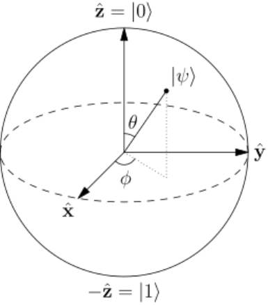
86
Figure 7. Bloch sphere: a geometrical representation of a qubit.
Note: The qubit is a two-state system which can be in a superpositional state similar to
Youngs classical experiment (Østgård et al., 2014).
The qubit requires a completely new way of thinking about information and
computation. A qubit is a two-level quantum mechanical system and it can be in a
superpositional state, i.e., multiple states at the same time. Mathematically, a quantum
logical qubit state can be written as a linear combination (viz., superposition) of |0 and
|1. Moreover, a qubit can be visually represented as a Bloch sphere which is
eponymously named after its inventor (Bloch, 1946). Fascinatingly, a single qubit can in
principle carry the information of all libraries in the world (Muthukrishnan & Stroud,
2000), viz., continuous-valued quantum information in a linear superposition (the
problem is how to measure the information without destroying it via collapse of the
superposition caused by the measurement).
The primary difference between one- and two-qubit states is their dimensionality. While
a one-qubit state has two dimensions a two-qubit state has four dimensions. This is the
case because in mathematics the tensor product A B (where signifies the tensor

87
product, also known as Kronecker product
58
) of two vector spaces A and B forms a new
higher-dimensional vector space which has a dimensionality equal to the product of the
dimensions of the two factors. In linear algebraic notation this can be written as
follows:
59
00
1
0
1
0
=
1
0
0
0
, 01
1
0
0
1
=
0
1
0
0
,
10
0
1
1
0
=
0
0
1
0
, 11
0
1
0
1
=
0
0
0
1
.
However, the two-qubit states which cannot be simply reduced to the Kronecker
product of single-qubit states because they are in an entangled state and the contained
information is not reducible to the individual constituent qubits (i.e. the whole is more
than the sum of its parts). The contained information is rather stored in the correlation
between the two states, i.e., it is non-local quantum information (Nielsen & Chuang,
2010). This non-locality of information is a crucial criterion which distinguishes
quantum computation from classical computation. Moreover, this type of non-local
information storage is the basis of various quantum protocols, for instance quantum
teleportation (Gottesman & Chuang, 1999).
A qutrit is defined as a unit of quantum information that is composed of the
superposition of three orthogonal quantum states (Klimov, Guzmán, Retamal, &
Saavedra, 2003). While a qubit is analogous to a classical bit, a qutrit is analogous to the
58
Note that the Kronecker product is not identical to usual matrix multiplication which is a different
mathematical operation.
59
Matrix-notation adapted from Microsoft's Quantum Development Kit: https://docs.microsoft.com/en-
us/quantum/quantum-concepts-5-multiplequbits

88
classical trit (trinary digit), for instance as utilised by ternary
60
computers based on
ternary logic (aka. 3VL) (Putnam, 1957). Consequently, a multiqubit quantum computer
with ≈300 entangled qubits could instantaneously compute more calculations than there
are atoms in the known universe. However, due to decoherence, superpositions are
extremely delicate. The problem lies in measuring the contained information. As soon
as an invasive measurement on the system is performed, the superpositional states
collapse into an eigenstate (environmentally-induced decoherence) and the information
is lost.
61
In sum, superposition is an essential property which is utilised for quantum
computation and it also appears to be applicable to models of cognition (Busemeyer &
Bruza, 2012). Moreover, the future of the rapidly developing fields of machine learning
and artificial intelligence is likely based on these extremely powerful quantum
computational principles which require a radically new way to think about information
(Biamonte et al., 2017; Dunjko & Briegel, 2017; Prati, 2017). Therefore, cognitive
psychology is now carrying the burden of proof: Why should nature not make use of
these extremely effective quantum-principles in the domain of cognitive processes?
Most models of cognition are strongly influenced by the principles of digital binary
computation (Piccinini & Bahar, 2013), although some argue that “cognition is not
computation”
62
(Bringsjord & Zenzen, 1997). A classical bit can adopt two possible
states (i.e., binary states) usually symbolised as 0 and 1 (but more generally “true” or
60
For instance, in “The art of computer programming” Donal Knuth (creator of TeX which forms the
basis of LaTeX) explains that in balanced ternary, every digit takes on one of 3 values, i.e., [−1, 0, +1]
(which can be more parsimoniously notated as [− ,0, +]). In the context of ternary notation, he also writes
that “Positional number systems with negative digits have apparently been known for more than 1000
years in India in Vedic mathematics” (Knuth, 1973, p. 192).
61
First attempts have been made to create qudits which, in contrast to two-state qubits can have multiple
states simultaneously. A qudit based quantum computer with two 32-state qudits, could compute as many
calculations as 10 qubit quantum computer, thereby speeding-up computation and significantly reduce
problems associated with the delicate entanglement of multi-qubit systems (Neeley et al., 2009).
62
Specifically, the authors argue that “computation is reversible; cognition isn’t; ergo, cognition isn’t
computation” (Bringsjord & Zenzen, 1997, p. 285). The irreversibility of cognitive processes might be
rooted in the stochastic nature of quantum processes (Aaronson, Grier, & Schaeffer, 2015; cf. Yearsley &
Pothos, 2014).
89
“false” or any other dichotomous notation, e.g., cats and dogs, as the physical substrate
in which the bit is realised is not important. This substrate independence is known as
multiple realizability, for a discussion of this fundamental concept see Shapiro (2000).
This implies that computation should be treated as logical abstraction – what is
important is software (logic) not the physical substrate (hardware).
Alan Turing wrote:
“The [Babbage Engine's] storage was to be purely mechanical, using wheels and cards.
The fact that Babbage's Analytical Engine was to be entirely mechanical will help us rid
ourselves of a superstition. Importance is often attached to the fact that modern digital
computers are electrical, and the nervous system is also electrical. Since Babbage's
machine was not electrical, and since all digital computers are in a sense equivalent,
we see that this use of electricity cannot be of theoretical importance. ... If we wish to
find such similarities we should look rather for mathematical analogies of function.”
Richard Feynman argued in his lecture series on quantum computation that Turing’s
arguments were impeccable but that he did not consider substrates that behave
according to the “strange” laws of quantum logic. The crucial point is that it has become
very clear that classical notions of physics are no longer defendable on empirical
grounds (e.g., local realism) (Giustina et al., 2015; Hensen et al., 2015; Wiseman,
2015). All information processing systems are embodied in some form of physical
substrate. Given that those physical substrates ae governed by the laws of quantum
mechanics, it follows that classical (Newtonian) notions of computation have to be
revised (and in fact are currently being revised) in the light of insight derived from
quantum physics. For instance, Google and NASA are currently heavily investing into
quantum computation and quantum AI (both are grounded on quantum logic). In sum,
90
quantum computational principles will significantly speed up a large array of
computational processes (Rønnow et al., 2014) and might turn out to be a driving force
for the continuation of Moore’s law (Lundstrom, 2003; G. E. Moore, 1965).
Superposition and entanglement are pivotal concepts in quantum information and
quantum computing (Boyer, Liss, & Mor, 2017). Quantum information and
computation are closely related to quantum cognition, as cognition is understood to be
information processing. Many cognitive and neuroscientists believe that cognition is
essentially a form of computational, i.e., it can be modelled mathematically by utilising
various computational principles (i.e., Bayes’ rule). Therefore, it is obvious that
cognitive scientists should consider quantum computational principles which do not
obey Bayes’ rule (which is based on Kolmogorov’s probability axioms). The same
quantum computational principles are also important for neuroscience and particularly
(neuro)computational neuroscience and artificial intelligence. Currently, neurons are
almost exclusively modelled as binary states (firing vs. resting), even though several
researchers are now beginning to integrate quantum approaches into their efforts
(Schuld, Sinayskiy, & Petruccione, 2014). From a quantum perspective, neurons can be
modelled as superpositional states. Given that neurons are thought to underpin all of
cognition (at least in a reductionist materialism framework) this has implications for the
high-order cognitive processes and computational models of cognition which are based
on these neurocomputational processes.
1.8 Perceptual judgments under uncertainty
Random walk models (e.g., Ratcliff & Smith, 2004; Usher & McClelland, 2001) which
focus on reaction times in various decision scenarios assume that evidence
(information) is accumulated diachronically (over time) until a specific critical decision-
91
threshold (or criterion) is reached (Busemeyer & Bruza, 2012). In these models, the
weights associated with each option increases chronologically in a progressive manner.
However, at each discrete point in the temporal sequence the system is assumed to be in
a definite determinate state. This state can in principle be accessed by taking a
measurement. Moreover, it is assumed that the act of measuring does not influence the
state under investigation. That is, classical models presuppose that 1) a given system is
consistently in a specific state (even though the observers’ cognition of this state might
be uncertain) and 2) that this state is independent of the measurement operation which is
performed on the system. Prima facie, these postulates seem intuitive and logically
valid. How else could one build a model of a system if it is not in a definite (stable)
state at any point in time? And how else could one gain “objective” information about
the state of the system if not via independent (interference-free) measurements which
“read-out” the actual state of the system?
However, both assumptions stand in sharp contrast with one of the main ideas of
quantum probability (QP) theory which provides the axiomatic basis of quantum theory.
A fundamental insight derived from quantum theory is that taking a “physical
measurement” of a “physical system” actively creates rather than passively records the
property under investigation. By contrast, classical theories assume that taking a
measurement merely reads out an already pre-existing state of a system.
Moreover, QP is incompatible with the classical notion that a given system (be it
physical or psychological) is always in an a priori determinable state at any point in
time. By contrast, QP allows for the possibility that a system can be in a superpositional
state in which n possibilities can exist simultaneously. It is only when a measurement is
taken that these undetermined potentialities collapse into determinate actualities.
The collapse of the wave-function Ψ is caused by interactions with the environment, a

92
process known as decoherence, i.e., the destruction of interference (Zurek, 1994). This
environment-induced collapse causes a loss of information, i.e., entropy.
63
In other
words, decoherence is the transition from a quantum state to a classical state, a process
called “Einselection” (Zurek, 2003). Thus, Einselection imposes classicality via a
drastic reduction of the dimensionality of the Hilbert space, in other terms, it creates
coherence from decoherence (Zurek, Habib, & Paz, 1993). That is, “classical structure
of phase space emerges from the quantum Hilbert space” and “in measurements,
Einselection replaces quantum entanglement between the apparatus and the measured
system with the classical correlation” (Zurek, 2003, p. 715). Our foregone discussion of
the concept of complementarity in visual perception illustrates this point. The Rubin’s
vase can be regarded as a bistable superpositional quantum state. The visual percept is
in a superpositional state and it is only when a measurement is taken (i.e., an observer
observes the stimulus) that the superposition collapses into a mutually exclusive
“either/or” eigenstate (the dominance of either foreground or background) caused by the
process of Einselection. Similarly, the Necker cube (Necker, 1832) has been described
in terms of quantum superposition and temporal nonlocality
64
(Atmanspacher & Filk,
2010; Atmanspacher, Filk, & Römer, 2009; Conte, Khrennikov, Todarello, Federici,
Mendolicchio, et al., 2009) and the quantum Zeno effect (Asher Peres, 1980) has been
successfully applied to model the switching rates between bistable (ambiguous) visual
percepts (Atmanspacher & Filk, 2013; Atmanspacher, Filk, & Römer, 2004).
We created two websites with additional information. One contains a dynamic
63
Entropy is a function of t (time evolution of the system) and a functional of the systems initial
state. The entanglement between the system and the environment can be calculated by computing the
entropy using the following intuitive algorithm (but see Zurek et al., 1993):
() = Tr (
()log
())
64
Locality describes the notion that a given event X cannot cause a change in Y in less time than =
/, where T signifies time, D is the distance between X and Y, and c the (constant) speed of light, and.

93
“Adobe® Shockwave Flash” animation of the Necker cube from a quantum cognition
perspective
65
. The other contains several digital animated artworks we designed and is
entitled “Necker Qbism: Thinking outside the box – getting creative with the Necker
cube”, in analogy with the superpositional quantum qubit and the concept of
simultaneity in cubism (Fry, 1988).
66
Briefly, Atmanspacher et al. applied the concept of “temporal nonlocality” (Brunner,
Cavalcanti, Pironio, Scarani, & Wehner, 2014) to the perception of bistable stimuli (i.e.,
the Necker cube). Temporal nonlocality implies that “events cannot be uniquely fixed in
time” and it is based on temporal Bell inequalities (or Leggett–Garg inequalities). The
exact definition of TBI goes beyond the scope of this chapter (but see Eberly, 2002).
Temporal Bell inequalities are particularly important for quantum-like context effects,
quantum entanglement, and the Kochen-Specker theorem (Santos, 2016). Within the
context at hand, temporal Bell inequalities are most pertinent when multiple
measurements are performed at different points in time. According to physical realism
67
(A. J. Leggett, 2014), a given system with two or more possible states is at all times in a
definite (fixed) state. Such a realist system satisfies the temporal Bell inequality
(Yearsley & Pothos, 2014). In the history of science, the violation of TBI is one of the
most important findings of the 20
th
century. The violation of TBI has first been
empirically demonstrated by Aspect, Grangier, & Roger (1981) and various
independent labs replicated and extended this paradigm-changing experimental
65
URL associated with the “Quantum Necker cube”: http://irrational-decisions.com/?page_id=420
66
URL of the “Necker Qbism gallery”: http://irrational-decisions.com/?page_id=1354
67
Physical realism postulates a mind-independent reality that is composed of physical entities that are
located in space and time, and interact causally with each other (Ellis, 2005). The concept is crucial for an
understanding of quantum physics as it forms the basis for many discussions among scholars, e.g., the
prototypical Einstein vs. Bohr debate on epistemology and ontology (Mehra, 1987).

94
finding.
68
The wide ramifications of this scientific finding are staggering because the
violation of TBI negates the fundamental concept of “local causality” – thereby ruling
out a large class of previously widely accepted physical models (Yearsley & Pothos,
2014), namely those which are based on local realism. However, in physics, local
realism has now been conclusively rejected (Giustina et al., 2015; Gröblacher et al.,
2007; Hensen et al., 2015). To those scientists who still persistently “believe” in an
objectively existing material reality
69
we recommend the concise NATURE article
entitled “The mental universe” authored by Richard Conn Henry, academy professor of
physics and astronomy at Johns Hopkins University (Henry, 2005) and the more recent
NATURE paper “Death by experiment for local realism” (Wiseman, 2015). In yet another
NATURE paper the following explicit statement has been formulated: ”Most working
68
Critics argue that the experiments might be confounded (e.g., by a loopholes/additional assumptions).
However, recent experiments successfully addressed these potentially confounding loopholes (e.g.,
Giustina et al., 2015) and provide strong empirical evidence of TBI violations, thereby paving the way for
implementing “device-independent quantum-secure communication” (Hensen et al., 2015). A even more
recent cutting edge experiment performed a “Cosmic Bell Test” by investigating violations of Bell
inequalities in polarization-entangled photons from distant Milky Way stars in real-time (Handsteiner et
al., 2017). The experiment confirmed the quantum theoretical prediction regarding statistical correlations
between measurements and provides further evidence against the classical local-realist theory. The
authors concluded that their experimental design rules out “any hidden-variable mechanism exploiting the
freedom-of-choice loophole” because it “would need to have been enacted prior to Gutenberg’s invention
of the printing press, which itself predates the publication of Newton’s Principia”. Interestingly, the
researchers report p-values < 1.8 x 10
-13
in support of their conclusion (Handsteiner et al., 2017, p. 4),
indicating that frequentist p-values are unfortunately still relevant in cutting-edge physics. The reporting
of such extremely small p-values (in the abstract) is misleading, as it capitalizes on the “replication
fallacy”, i.e., the widely shared fallacious belief that small p-values indicate reliable research (e.g.,
Amrhein, Korner-Nievergelt, & Roth, 2017).
69
Bishop Berkeley’s statement “esse est percipi (aut percipere)” — to be is to be perceived (or to
perceive) is relevant in this context. Samuel Johnson famously asserted in 1763 to have disproven
Berkeley's nonmaterialistic stance by kicking a rock and he is known to have said "I refute Berkeley
thus”, a non sequitur (cf. Priest, 1989; “Primary qualities are secondary qualities too”). This logical
fallacy goes by the name “argumentum ad lapidem” (Latin for “appeal to the stone”) (Winkler, 2005) as it
is no valid argument but merely superficially dismissing Berkley’s claim without providing any reasons
(Pirie, 2007). An example of this type of logical fallacy follows:
Person 1: Under the code name MK-Ultra, the CIA conducted illegal drug experiments on countless
nonconsenting human being to investigate mind control techniques which resulted in several deaths.
Person 2: This is just a conspiracy theory!
Person 1: Why do you think so?
Person 2: It is obviously just paranoia.
In this example of an “appeal to the stone” fallacy, Person 2 provides no logical reasons or facts. Person 2
merely asserts that the claim is absurd and therefore commits the same logical fallacy as Berkley’s
argumentative opponent..

95
scientists hold fast to the concept of 'realism' - a viewpoint according to which an
external reality exists independent of observation. But quantum physics has shattered
some of our cornerstone beliefs.” The authors go on and state that experimental
evidence (i.e., violation of Bell inequalities) has rendered “local realistic theories
untenable” (Gröblacher et al., 2007).
70
Similarly to the breakthrough in quantum
physics, an experimental demonstration of a TBI violation in psychological observables
would herald a paradigm-shift in psychology because such a finding would rule out a
large class of cognitive models which assume that cognitive systems are always in a
deterministic state (Yearsley & Pothos, 2014). Experimental approaches that could
falsify TBI in the context of visual perception have already been formulated
(Atmanspacher & Filk, 2010). The implications such an empirical discovery would have
for psychology and neuroscience cannot be overemphasised as the violation of BI is one
of the most thought provoking finding physics has ever made. The rejection of local
realism is not only highly counterintuitive, it might also “feel” very uncomfortable
because our common-sense worldview is firmly anchored in this most constitutive
paradigm. Such a finding would certainly cause severe cognitive dissonance in the
minds of majority of scientists (Festinger, 1957, 1962). That is, if results from quantum
physics challenge our most fundamental beliefs and force us to rethink reality, this can
70
At this point it is important to differentiate between classical (spatial) Bell inqualities (BI) and temporal
Bell inequalities (TBI), i.e., Bell's theorem for temporal order (Paz & Mahler, 1993; Zych, Costa,
Pikovski, & Brukner, 2017) This difference is directly related to the Heisenberg uncertainty principle
(Heisenberg, 1927) which asserts a fundamental limit to the precision of measurements.
ΔxΔp≥h/4π, where h is Plancks constant.
Specifically, this principle describes a mathematical inequality which states that complementary variables
(i.e., complementary physical properties such as position x and momentum p) cannot be simultaneously
known (observed/measured) with an arbitrarily high degree of precision. It is important to emphasise that
this principle is completely independent of the inaccuracy of the measurement device or any other
experimental variables (e.g., noise, unknown experimental confounds, etc.). Rather, the uncertainty
principle is fundamental to the nature of the quantum mechanical description of reality. The
Heisenbergian uncertainty principle constitutes one of the defining difference between spatial and
temporal Bell inequalities as the constraint does not apply when two measurements are performed at the
same point in time on two different particles located in different space points. On the other hand, it does
constraint the ability to resolve the two states in a second measurement at a later time on the same particle
(Calarco, Cini, & Onofrio, 1999).

96
evoke strong emotional/affective responses and various cognitive defence mechanisms
might be activated to protect our conceptual schemata from the radical (Bayesian)
revision of beliefs which is necessary when these finding and their implications are
taken seriously. The well-studied phenomenon of belief-bias is relevant in this regard.
Belief-bias a phenomenon in the psychology of thinking and logical (syllogistic)
reasoning which demonstrates that reasoning is biased by a priori beliefs, even though
the logical argument might be syntactically valid (i.e., logically sound). This conflict
between semantic believability (a System 1 process) and syntactical logical validity (a
System 2 process) leads to large proportions of fallacious conclusions when these aspect
are incongruent, viz., the conclusion of a given argument is logically valid but
semantically unbelievable according to priors beliefs (J. St. B. T. Evans, Barston, &
Pollard, 1983; Kahneman, 2003; Tsujii & Watanabe, 2009). A more detailed description
of belief-bias can be found in Appendix A6. Hence, for proper scientific thinking it is
important to counteract this systematic belief-bias in order to deduce logically valid
conclusions.
There is general consensus
71
(i.e., a strong prior belief) in cognitive psychology and the
neurosciences that cognitive processes are ultimately reducible to neuronal processes, a
perspective which goes by the name of “materialistic reductionism” (however, this
71
Group-consensus (conformity) is another important factor which can dramatically distort the validity of
scientific judgments and reasoning (Asch, 1955). Social-identity theory (Tajfel & Turner, 1986) is yet
another powerful explanatory theoretical framework in this respect. If the social identity of a given
scientists (or a group of scientists, or a whole scientific discipline) is based on the (untested) assumption
of local realism, then any evidence which challenges this shared Weltanschauung is perceived as a threat
to the group norm. These group processes are in conflict with rational and “objective” scientific
reasoning. These well-documented effects are based on complex social dynamics which cannot be
ignored in the context of scientific reasoning. The “need to belong“ (Baumeister & Leary, 1995) is a
fundamental human motive which (implicitly) motivates much of human behaviour. Scientists (and the
groups they affiliate with) are no exception. Awareness of these confounding effects on reasoning and
decision-making is crucial but usually exclusively taught as part of a specialised social psychology
curriculum, which is (dis)regarded as a “soft” science even though it uses the same quantitative methods )
as other disciplines, e.g., the biomedical sciences (to be precise, a loically incoherent hybrid between
Fisherian and Neyman-Pearsonian hypothesis testing, but see Gigerenzer, 1993).
97
conceptual paradigm is not based on empirical evidence – it is merely hypothetical).
Therefore, the notion of realism (as used in physics) is an almost unquestioned
assumption of all mainstream cognitive (and neurological) models. An interesting
question is the following: If TBI is violated at the cognitive process level, but the brain
is assumed to be classical, then what exactly is the substrate of the quantum process
(Yearsley & Pothos, 2014)? And what role do quantum processes play in
neurophysiology/neurochemistry (Baars & Edelman, 2012; Koch & Hepp, 2006)?
Recently, several quantum models of the brain have been proposed. The most widely
known (and most controversial) theory is the “Orchestrated objective reduction” (Orch-
OR) hypothesis formulated by Sir Roger Penrose and Stuart Hameroff which postulates
that quantum processes at the neuronal microtubular level are responsible for the
emergence of consciousness. Appendix A2 provides a synopsis of the conjectural Orch-
OR quantum-brain hypothesis.
1.9 A real-word example of superposition and collapse
The generic probability framework developed in quantum physics appears to be relevant
to multifarious psychological processes (Atmanspacher & Römer, 2012). Especially, the
concept of noncommutativity appears to be pertinent for cognitive operations.
Noncommutativity, in turn, is closely related to superposition and the collapse of the
wave-function. The following paragraph provides an intuitive simplistic illustration of
the principle of superposition applied to a real-world decision-making scenario.
Subsequently, we will discuss the concept in somewhat more technical terms in the
context of visual perception.
Here is the real-world example in the context of academic decision-making: Suppose an
examiner has to decide whether a Ph.D. thesis should be passed or failed. From a

98
classical information processing point of view the response format is binary, i.e., either
yes or no response (lets denote this with 1 or 0), a dichotomous decision. These values
might change dynamically over time as the examiner reads the thesis, but at any
moment in time, the associated cognitive variable is assumed to be in a definite fixed
state (see Figure 8). However, contrary to the classical notion, it seems plausible that the
examiners cognitive state does not jump from one discrete binary state to another (like a
flip-flop or an electron jumping from one orbit to another). Instead, the examiner might
experience ambiguity about both states simultaneously (see Figure 9). That is, until a
final decision is made, the cognitive system is in a superpositional state, i.e., an
indeterminate state. When the decision is finally reached (e.g., no corrections, i.e., 0),
the superpositional 1/0 state instantly transforms into a determinate state. This is the
simplified basic tenet of superposition and collapse in QP theory, explained in the form
of an intuitive analogy.
Observe state i at time t where p
i
= probability of state i
p(t | i) = [1,0,..,1,..0]'
p(t + s) = T (s) p(t | i)
Figure 8. Classical sequential model (Markov).
Observe state i at time t where ψ
i
= amplitude of state i
ψ (t | i) = [1,0,..,1,..0]'
ψ (t + s) =U(s) ψ(t | i)
1
0
1
0
1
1
0
0
(t)
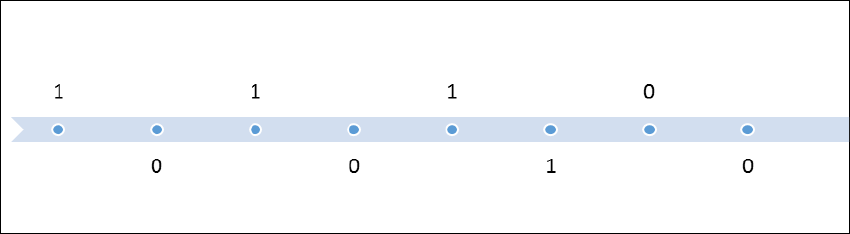
99
Figure 9. Quantum probability model (Schrödinger).
This example illustrates the concept of “quantum indeterminacy” (Busch, 1985; cf.
Glick, 2017) which stands in direct contrast with deterministic physical theories which
predate quantum physics. Deterministic theories assumed that:
1) a given (physical) system always has a in principle determinable state that is
precisely defined by all its properties.
2) the state of the system is uniquely determined by the measurable properties of the
system (i.e., the inverse of point 1).
Thus, an adequate account of quantum indeterminacy needs to operationalise what
constitutes a measurement – an unresolved “hard” problem which we will address in
greater detail in the general discussion section.
1.10 Determinism vs. constructivism
“The procedure of measurement has an essential influence on the conditions on which
the very definition of the physical quantities in question rests.” (Bohr, 1935, p.1025).
According to the theoretical nexus of quantum cognition, superposition,
noncommutativity, and complementarity are closely interlinked phenomena. To reiterate
the basic principles of QP in more technical terms, superposition defines a state which
has a specific amplitude across >1 possibilities. QP postulates that taking a
1
0
0
0
0
1
1
1
(t)

100
measurement causes a continuously distributed state to collapse into a discontinuous
discrete state (via wave function collapse as described by Schrödinger’s wave-
equation). That is, the quantity being measured changes from a superimposed state into
an Eigenstate.
72
The crucial difference to sequential Markovian data models (e.g.,
Camastra & Vinciarelli, 2015) is the impossibility to create what Schrödinger called an
“Erwartungskatalog” (expectation catalogue), i.e., an index of the trajectory of states of
the system as a discrete time-series. Note that it is only when a measurement is taken
that a discrete value is created via collapse of Ψ. The trajectory of the state of a quantum
system is called a “quantum trajectory” (Sanz & Borondo, 2007) and can be
conceptualised as stochastic random walk
73
in a multidimensional Hilbert space.
However, in contrast to classical random walk models, the evolution of the quantum
system is conditioned upon measurements. In the current context of perceptual
judgments, we are particularly interested in the question whether the perceived
luminance level of a visual stimulus changes depending on whether there was an
antecedent psychophysical measurement or not. Let us assume that the perceptual
evaluation is developing over two stages. Each stage entails the presentation of a visual
stimulus (a grey rectangle with high or low luminance levels). From a classical
probability (CP) perspective, it should not make any difference if the percipient is
requested to provide a perceptual evaluation just after the second stage or after the first
stage as well. If an intermediate evaluation is required, this is assumed to merely read-
out an already pre-existing internal visual percept and therefore this should not have any
impact on the final perceptual judgment in the second stage. By contrast, from QP
perspective, a perceptual evaluation (an introspective measurement) can significantly
72
The word “Eigenstate” is derived from the German word “Eigen”, meaning “own”, “inherent”, or
“characteristic”.
73
The term „random walk“ was first introduced by the English mathematician and biostatistician Karl
Pearson in a seminal N
ATURE article entitled „The Problem of the Random Walk“ (Pearson, 1905).

101
change the state of the percipients’ cognitive system (the cognitive state vector is
realigned). Ergo, the intermittent perceptual judgment (i.e., cognitive measurement) can
causally interfere with the result of the subsequent judgement. Note that the CP model
does not predict any order effects due to an interjacent measurement whereas the QP
model predicts such effects a priori. Of course, it is possible to explain such a finding in
classical terms with auxiliary hypotheses (Leplin, 1982) which can be added a
posteriori to the CP model in order to provide a post hoc explanation for this kind of
carry-over effect. However, this can only be accomplished by adding additional
components to the model which are not inherent to CP theory and which have not been
predicted a priori. Consequently, according to the law of parsimony, i.e., Ockham's
razor (Rodríguez-Fernández, 1999), the QP model should be preferred over the CP
model.
74
1.11 Quantum logic
The claim that logic should be subject to empirical research was first articulated by von
Neumann and Birkhoff in the Annals of Mathematics (Birkhoff & Neumann, 1936).
This position was later also advocated by Hilary Putnam (Cartwright, 2005; Maudlin,
2005). He argued that in the same way as non-Euclidean geometry revolutionised
geometry, quantum mechanics changed the fundamental assumptions of logic. In his
seminal paper entitled “Is logic empirical”, Putnam proposed the abandonment of the
algebraic principle of distributivity, a position which has been challenged on several
74
Note that CP and QP theory are not necessarily mutually exclusive. Classical probability is a special
case within the more general overarching (unifying) quantum probability framework.

102
grounds (Bacciagaluppi, 2009; Gardner, 1971). The distributivity principle has received
great attention in the context of irrational reasoning (Hampton, 2013; Sozzo, 2015), for
instance, in the context of the conjunction fallacy (e.g., the Linda paradox
75
). However,
while violations of the distributivity principle are inconsistent with classical logic, they
are entirely consistent in the axiomatic framework and various prima vista seemingly
irrational reasoning fallacies have been successfully modelled using quantum logic
(Moreira & Wichert, 2016b). A pivotal difference from classical Boolean algebra is
described by the von Neumann’s concept of “simultaneous decidability” and extension
of simultaneous measurement. Birkhoff’s and von Neumann's interpretation of quantum
mechanics have been extensively discussed in philosophy of science, inter alia, by Karl
Popper (Popper, 1968).
In the psychological literature, classical probability theory dominates all modelling
efforts. That is, almost all cognitive and neuroscientific models implicitly assume the
validity of classical probability theory. The standard model of probability (known as
Boltzmann/Gibbs distribution in physics or Kolmogorov’s laws in classical probability
theory) is based on the set-theoretic assumption that probabilities always add up to 1.
This is formally axiomatized in the law of conditional probability. The Kolmogorov
formulation is as follows (Kolmogorov, 1956):
75
A prototypical version of Linda paradox goes as follows (Tversky & Kahneman, 1983):
Linda is 31 years old, single, outspoken, and very bright. She majored in philosophy. As a student,
she was deeply concerned with issues of discrimination and social justice, and also participated in
anti-nuclear demonstrations.
Which is more probable?
a) Linda is a bank teller.
b) Linda is a bank teller and is active in the feminist movement.
(We ask the reader to answer the question before reading the following paragraph.)
The majority of respondent “irrationally” choose option b) over option a). However, the conjunction of
both events occurring together is probabilistically less than or equal to either event occurring in isolation.
This inequality can be formalised as () () and () ().

103
Equation 5. Kolmogorov’s probability axiom
(|) =
()
()
Current cognitive and decision models are almost exclusively derived from the
Kolmogorov axioms (Kolmogorov, 1933/1950). Quantum probability is based on
fundamentally different mathematical axioms and has the potential to provide a viable
alternative to the dominant Kolmogorovian paradigm
76
.
1.12 Noncommutative decisions: QQ-equality in
sequential measurements
In the current experimental context, the most relevant difference between classical and
quantum probability models is the way in which they deal with violations of the
commutativity axiom (the quantum model allows for violations of symmetry, that is,
observables do not have to commute). In other terms, the defining difference between
classical probability theory and quantum probability theory is noncommutativity of
operators.
77
If projectors do commute, classical probability theory applies, “iff” they do
not commute, quantum probability applies. Accordingly, quantum theory is only
applicable in cases of noncommutativity (Busemeyer & Bruza, 2012), otherwise it is
identical to the classical probability framework. Quantum stochastic calculus is the
76
Bose-Einstein statistics are another counterintuitive instance of quantum probabilities which are
incongruent with classical notions of probability (quantum dice). The details go beyond the scope of this
chapter. However, for the curious reader, we created a website which contains additional information on
this topic: http://irrational-decisions.com/quantum_dice/
77
In matrix algebra, the product of matrices does not necessarily commute, for instance:
[
0 2
0 1
] = [
1 1
0 1
] [
0 1
0 1
] [
0 1
0 1
] [
1 1
0 1
] = [
0 1
0 1
]
In matrix algebra, every subspace corresponds to a projector, i.e., the projector is an operator that takes a
vector and projects it onto the subspace (Busemeyer & Bruza, 2012) and projector A multiplied by
projector B does not always give the same result as projector B times projector A.

104
mathematical framework which is used to model the random
78
evolution of quantum
systems undergoing measurements. It is a generalization of stochastic calculus to
noncommuting observables (Hudson & Parthasarathy, 1984).
Equation 6. Classical probability theory axiom (commutative).
() = ()
Equation 7. Quantum probability theory axiom (noncommutative).
|
|
|
| |
|
|
|
How do we transfer this abstract mathematical formalism to actual real-world
phenomena? Let us consider a representative realistic example: In a Gallup poll
conducted in 1997, half of the sample (n = 1002) was asked, “Do you generally think
Bill Clinton is honest and trustworthy?” and subsequently they were asked the same
question about Al Gore (Moore, 2002). Using the standard (random) split sample
technique, the other 50% of respondents answered exactly the same questions but the
question order was reversed. When the question about Clinton was asked first, he
received a 53% agreement whereas Gore received 76% (Δ 23%). However, when the
78
Werner Heisenberg differentiates between objective randomness and subjective randomness. While the
outcome of throwing two die is subjectively random, quantum randomness is objectively random. In
principle, the ooutcome of throwing a die could be determined – however the Newtonian dynmics are just
to complex (viz., Laplace's omniscient demon could in principle predict the outcome). Quantum
randomness is by its very nature indeterminstic and therefore not dependent on the epistemological state
of the observer (e.g., unknown hidden variables). To twist Einsteins famous words: God does play
quantum dice, i.e., at its most fundamental level nature is indeterministic. This empirical fact poses a
serious problem for mechanistic causal models across the sciences. Specifically, because the demarcation
criterion between “quantum vs. not quantum” (i.e., micro vs. macro) appers to be arbitry (Arndt et al.,
1999; Van der Wal et al., 2000). That is quantum effects are observed in macro scale molecules and
eminent physicists argue that there is theoretically no upper limit to the size of object which obey
quantum laws (Zeilinger, 2012).

105
question order (the order of sequential measurements) was inverted Clinton received
59% while Gore received only 67% (Δ 8%).
Figure 10. Noncommutativity in attitudinal decisions.
Classical probability theory cannot account for this kind of order effects because events
are represented as sets and are stipulated to be commutative, that is, P (A ∩ B) = P (B ∩
A). That is, the empirically observed order-effects clearly violate the Kolmogorovian
commutativity axiom. Quantum models of cognition can account for these prima facie
"irrational" judgment and decision-making phenomena and indeed predict them a
priori. In the pertinent literature, the effect of posing attitude questions successively in
different orders has been termed QQ-equality, i.e., quantum question equality (Z. Wang,
Solloway, Shiffrin, & Busemeyer, 2014). This measurement effect has been
investigated in a large scale meta-analytic study (based on 70 national representative
surveys each containing between 600-3000 participants). The results provided strong
support for the predicted QQ equality. Similar results in support of the broad
applicability of QQ-equality to cognitive processes have been obtained in various
unrelated domains, for instance, in dynamic semantics (beim Graben, 2013), thereby
Clinton
53%
Gore
67%
Gore
76%
Clinton
59%

106
supporting the generalisability of QQ-equality across multiple domains of inquiry.
79
Taken together, these findings suggest that QP, originally developed to explain
noncommutativity of measurements in quantum physics, provides a desirably
parsimonious explanation for measurement order effects in the social, behavioural, and
cognitive sciences (Z. Wang & Busemeyer, 2013). Classical Bayesian
80
and Markov
models are unable to account for QQ-equality and are thus incapable of explaining the
empirical data. In the quantum probability framework events are subspaces in an n
dimensional Hilbert space and they may either be compatible or incompatible
(incompatible events are aligned orthogonal in respect to each other). In other words,
noncommutative order effects can be modelled in terms of incompatible projectors on a
Hilbert space (Z. Wang et al., 2014). If they are compatible, they can simultaneously
coexist without influencing each other. On the other hand, incompatible event, as
illustrated in the example above, interfere with each other, thereby causing order
interference effects. In quantum physics, these interference effects have been studied
extensively and the constructive role of measurements/observations is firmly established
even though the exact nature of what exactly defines a measurement/observation is a
wide-open question and is related to the measurement problem (Echenique-Robba,
2013). Several theorist argue that consciousness is crucial for the collapse of the wave-
79
QQ-equality was initially developed to account for noncommutativity of measurements in quantum
physics. However, multiple studies have demonstrated that the same principle is applicable to various
psychological processes. This can be regarded as a paradigmatic case of “scientific consilience” (E. O.
Wilson, 1998b), viz., evidence from unrelated sources support the same scientific theory. In other words,
converging evidence corroborates the generalisability of QQ-equality across multiple domains. QQ-
equality can be formalised as follows:
= [(AyBy) + (AnBn)] [(ByAy) + (BnAn)]
= [(AyBn) + (AnBy)] [(ByAn) + (BnAy)] = 0.
For mathematical details see the supplemental material provided by Wang et al., (2014) or the textbook
by Busemeyer & Bruza (2012).
80
Several lines of research combine Bayesian approaches with quantum logic. Combinatorial approaches
include the “Quantum Bayes Rule” (Schack, Brun, & Caves, 2001) and “Quantum Bayesian Networks”
(Low et al., 2014). Recently, “quantum-like Bayesian networks” have been utilised to model decision
making processes (Moreira & Wichert, 2016a) and it has been demonstrated that they are able to
parsimoniously accommodate violations of the laws of classical probability, for instance, the
comonotonic “sure-thing principle” (A. Y. Khrennikov & Haven, 2009).
107
function, thereby assigning consciousness a crucial role within the formal framework of
quantum physics (that is, localisable matter only exists when observed by a conscious
agent) (C. U. M. Smith, 2009).
In the context of the Gallup poll example described before, the quantum-like
constructive role of measurements can be described as follows: The cognitive state
constructed from the first question changes the cognitive context used for evaluating the
second question, i.e., the cognitive state vector is rotated, and a subsequent judgment is
based on this change in cognitive state. From a quantum cognition perspective, attitudes
are not simply retrieved from memory structures – they are constructed online or “on
the fly” (White et al., 2014b).
The quantum cognition approach can be regarded as a form of cognitive constructivism,
not to be confused with Vygotskian or Piagetian constructivism, although there are
significant conceptual similarities, i.e., the view of the cogniser as an active (rather than
passive) information processor and the emphasise on the contextual situatedness of
information processing (Barrouillet, 2015; Gerstenmaier & Mandl, 2001)).
In the cognitive sciences, the assumption that cognitive variables have a fixed value at
each moment in time is generally unquestioned and has hitherto been uncontroversial.
Cognitive variables might change diachronically (as a function of t) but at each specific
point in time the cognitive system is assumed to be in a definite state. This intuitions
appears to be common sense, however, scientific facts and our intuitions about reality
do not always coincide. An alternative way to look at cognitive variables is that
measuring cognitive variables is a constructive process which actively creates the
specific state of the variable under investigation. This implies that it is impossible to
create an index of the possible values of the cognitive variables at each and every point
in time (Yearsley & Pothos, 2014).

108
This notion is indirectly supported by recent neuroscientific simulation studies, which
focus on the energy dynamics of neural network structures (Sporns, 2014). From an
evolutionary and cognitive economy point of view, it seems to be very inefficient to
store a vast number of opinions about reality in our neuronal networks (e.g., sparse
coding of memory). Santiago Ramón y Cajal postulated over 100 years ago that our
neuronal morphology is shaped by “laws of conservation for time, space, and material”
(Cajal, 1895). Following this quasi-Helmholtzian line of thought, it seems plausible that
most of our opinions are constructed in real time
81
and do not exist a priori in a
determinate state in some (neural) substrate. The contextual constructivism postulated
by quantum cognition provides an elegant framework to formalize this intuition
(Busemeyer & Bruza, 2013).
1.13 Quantum models of cognitive processes
Recent findings in quantum cognition have challenged many of the most fundamental
assumptions about the basic characteristics of cognitive systems and they have led to the
development of a number of novel modelling approaches (Busemeyer & Bruza, 2012).
Quantum cognition introduces several completely new concepts to the field of
psychology which were previously not part of the scientific discourse within the
discipline. These novel concepts are superposition, entanglement, and incompatibility,
to name just the most important innovations. These novel concepts have provided fresh
insights into the nature of various cognitive processes (Aerts & Sassoli de Bianchi,
2015; Bruza, Busemeyer, & Gabora, 2009; Busemeyer, Pothos, Franco, & Trueblood,
81
It should be noted that answers to certain classes of questions are very likely retrieved from relatively
stable memory (network) structures rather than being contextually constructed (e.g., autobiographical
information).
109
2011a; Conte, Khrennikov, Todarello, Federici, & Zbilut, 2009; Segalowitz, 2009;
Sozzo, 2015; Z. Wang et al., 2013).
1.14 Contextualism, borderline vagueness, and Sôritês
paradox
One of the most widely cited arguments that motivates the application of QP to
cognitive phenomena is the existence of interference effects in higher-order cognitive
processes such as decision making and logical reasoning (Aerts, 2009; Blutner, Pothos,
& Bruza, 2013; Busemeyer, Wang, & Lambert-Mogiliansky, 2009). A recent
publication entitled “a quantum probability perspective on borderline vagueness”
(Blutner et al., 2013) discusses the importance of the concept of noncommutativity in
the context of decisions involving natural concepts. Natural concepts oftentimes lack
precisely defined extensions, for instance, what is the smallest size of a man called
“tall”? The demarcating criterion which differentiates between “tall” and “not tall” is
not clearly defined (Karl Popper struggled with the same “demarcation problem” in the
context of science versus pseudo-science). The authors investigated the fuzziness of
natural everyday concepts and compare various approaches (e.g., fuzzy logic). We
argue that similar to semantic concepts, visual categorisation is oftentimes ambiguous
and vague. Specifically, we argue that the fuzzy boundaries of natural concepts
described in other quantum cognition models are particularly applicable to visual
judgments. For instance, what is the lowest luminance level of a stimulus categorised as
“bright”? The absence of a modulus or “perceptual anchor” complicates the matter even
further. As with natural concepts, the demarcating boundaries between “bright” and
“not bright” are not clearly defined and it is often uncertain if the predicate applies to a
given visual stimulus (partly due to the imprecise definition of the predicate). It follows

110
that Sôritês paradox (also known as “the problem of the heap”) is extendable to visual
perception (and perception in general) especially in the context of the “just noticeable
difference”, JND (Norwich & Wong, 1997). Sôritês paradox (which has been ascribed
to the Greek philosopher Eubulides of Miletus) illustrates the vagueness of predicates
(Blutner et al., 2013). The paradox is based on the seemingly simple question: When
does a heap of sand become a heap?
82
The associated syllogistic argument can be
formulated as follows:
1
st
premise:
2
nd
premise:
Conclusion:
100000000000 grains of sand are a heap of sand.
A heap of sand minus one grain is still a heap.
Ergo, a single grain of sand is a heap.
Sôritês paradox as a syllogistic argument, i.e., modus ponens () ) ).
Repeated application of the minor premise (iterative removal of single grains of sand,
i.e., inferential “forward chaining”) leads to the paradoxical, but deductively necessary
(i.e., logically valid) conclusion that a single grain of sand is a heap. Figure 11
illustrates Sôritês paradox applied to visual perception. Adjacent luminance differences
(e.g., tick-mark 1 versus 2) are indistinguishable by the human visual system while
larger contrasts (e.g., tick mark 2 versus 3) are easily distinguishable.
82
The “Bald Man (phalakros) paradox” is another allegory which illustrates the vagueness of predicates:
A amn with a full head of hair is not bald. The removal of a single hair will not turn him into a bold man.
However, diachronically, continuous repeated removal of single hairs will necessarily result in baldness.

111
Figure 11. Sôritês paradox in visual brightness perception.
Conceptual vagueness has received a lot of attention from logicians, philosophers, and
psychologists (e.g., Eklund, 2011; Putnam, 1983; Serchuk, Hargreaves, & Zach, 2011).
Here we are particularly concerned with cases of borderline contradictions such as “X is
bright and not bright” where X denotes a borderline case (Blutner et al., 2013).
Specifically, the “superposition” of “bright” and “not bright” is relevant from a quantum
cognition perspective and it has been cogently argued in various psychological contexts
that this kind of superposition introduces cognitive interference effects (Aerts, 2009;
Aerts et al., 2011; Blutner et al., 2013). The postulated interference effects are
analogous to those observed in quantum mechanics (i.e., the principle of superposition).
The mathematical similarities have been discussed elsewhere (e.g., Busemeyer et al.,
2011a) and go beyond the scope of this chapter.
Importantly for the experimental context at hand is the fact that the concept “bright” is a
vague concept because the exact demarcation from “not bright” is arbitrary and
imprecise. When making perceptual judgments on a scale
83
ranging from “bright” to
“not bright”, the percipient is confronted with a large degree of indeterminacy
(especially when no absolute modulus is provided to anchor the judgment on the scale).
It has been convincingly argued that the logical principle of non-contradiction (i.e., the
semantic principle of bivalence
84
) does not necessarily hold true in such situations
(Blutner et al., 2013). Epistemological accounts of vagueness (Sorensen, 1991; Wright,
1995) consider vagueness as the consequence of nescience on part of the percipient and
83
For instance, as measured on a quasi-continuous psychophycial visual-analogue scale (Aitken, 1969).
84
The semantic principle (or law) of bivalence is closely related to the 3
rd
Aristotelian law of thought, i.e.,
the law of the excluded middle (principium tertii exclusi) which can be stated in symbolic notation as
. (), where ~ signifies negation (after Whitehead & Russell, 1910). We will discuss this logical
principle in greater detail in the context of quantum cognition in subsequent chapters because it plays a
crucial role for superpositional states (quantum logic).

112
not a fundamentally ontological problem (but see Daniliuc & Daniliuc, 2004).
Ontological accounts (e.g., contextualism), on the other hand, regard vagueness as a
case of context-sensitivity (Åkerman & Greenough, 2010; Greenough, 2003; S. Shapiro
& Greenough, 2005), i.e., the uncertainty associated with vagueness is regarded as a
contextual phenomenon. This kind of context-dependence has been designated as “v-
standards” and it describes any contextual parameter that is responsible for the
vagueness (Åkerman & Greenough, 2010; Blutner et al., 2013). Fuzzy set theorists
would agree with this ontological stance. They propose a form of logic which allows for
graded truth values (L. a. Zadeh, 1965; L. A. Zadeh, 2008). Alxatib & Pelletier (2011)
concluded that such borderline cases pose a serious problem for classical
(Kolmogorovian/Boolean) logic. However, Blutner et al., (2013) demonstrated that QP
provides a powerful explanatory framework for borderline contradictions (Blutner et al.,
2013). QP utilises vectors in a Hilbert space and it defines a linear operator on .
Specifically, a projection operator
85
is a linear operator which projects vectors to certain
subspaces of
86
. The underlying algebraic logic is non-Boolean in nature. Rather, it
obeys the logic of orthoalgebra (Dalla Chiara & Giuntini, 1995). A defining difference
between orthoalgebra and Boolean algebra is that the former does not obey the
distributive law which form the basis of the law of total probability. The law of total
probability, in turn, form the axiomatic basis for Bayes’ rule (Bayes & Price, 1763).
Ergo, QP is incompatible with Bayes’ rule. Crucially, in QP the order in which
85
Most psychologists are familiar with the General Linear Model and specifically multiple regression.
The squared length of the projection in quantum probability theory is equivalent to the R
2
in multiple
regression analysis, i.e., the coefficient of multiple determination (Busemeyer & Bruza, 2012).
86
If a given system is in state Ψ, then a measurement will change the state of the system into a state
which is an eigenvector e of A and the observed value λ will be the corresponding eigenvalue of the
equation A e = λ e. This description implies that measurements are generally non-deterministic. The
formulaic description for computing the associated probability distribution Pr on the possible outcomes
given the initial state of the system Ψ is as follows: Pr () = E (), where E(λ) signifies the
projection onto the space of eigenvectors of A with eigenvalue λ.

113
projection operators are combined can make a significant difference (Pothos &
Busemeyer, 2013). Two projection operators A and B in a given Hilbert space do not
necessarily have to commute. That is, QP allows for AB≠BA (Blutner et al., 2013).
However, if all projection operator commute, QP is equivalent to Boolean algebra.
Thus, Boolean algebra is a special case of quantum probability theory which provides
an overarching (more generalisable) axiomatic framework. We would like to emphasize
the difference as it is crucial for the experimental investigation at hand: The principle of
commutativity (or the violation thereof) is a critical criterion to differentiate between
Boolean logic and quantum logic. We will discuss this noncommutativity criteria in
greater detail in the context of constructive measurements of psychological observables.
In QP notation, the term ∂(A,B) is called the interference term. If ∂(A,B) is zero, A and B
commute (Blutner et al., 2013) otherwise A and B are non-Abelian
87
. In the context of
psychological borderline vagueness (Alxatib & Pelletier, 2011), which is notoriously
difficult to explain in a classical probability framework, it has been demonstrated that
the QP model provides a parsimonious explanatory model with an acceptable/good
index of fit, χ
2
(4)=5.47; p=0.24 (Blutner et al., 2013).
QP requires us to broaden and revise our conception of probability theory. QP is a much
more general axiomatic framework compared to classical probability theory because it
is able to describes all real-world properties (both at the micro and macro level). Some
hardliners argue that reality as a whole is quantum mechanical, i.e., the world (and the
whole universe) are a quantum system and that the underlying logical structure is based
on the axioms of quantum logic. However, every-day reality appears classical (i.e.,
87
In group theory, Abelian groups denote a group in which the application of a group operation to two
group elements is independent on the order in which the operation is performed (viz a commutative
group). In other terms, Abelian Groups (eponymously named after the mathematician Niels Hendrik
Abel) conform to the commutativity axiom in abstract algebra (Durbin, 1967).
114
Boolean/Kolmogorovian) to the naïve percipient, but this is only the case because
humans happened to almost exclusively perceive commuting observables (unless one
discovers quantum mechanics or tests psychophysical commutativity in controlled
empirical experiments). This naturally reinforces the “representativeness heuristic”
which has been extensively studied in the field of thinking and reasoning (Kahneman &
Tversky, 1972). In other words, numerous empirical encounters with commuting
variables shaped and moulded our representations, heuristics, and intuitions and created
the impression that commutativity is a constant nomological property of psychological
(and physical) observables. However, from a rationalist point of view, insights derived
from quantum mechanics require us to revise our most fundamental concepts of logic
and the associated mathematical models. This empiricist position was also advocated by
Quine, i.e., Quine argued that logic and mathematics are also subject to revision in the
light of novel experiences and he explicitly employed “deviant quantum logic” as an
example. In other words, Quine adopted initially an empirical quasi-Bayesian updating
approach to logic. However, Quine later changed his opinion on this topic and argued
that the revision of logic would be to essentially "change the subject”. Hilary Putnam
also participated in this fundamental debate about the empirical status of logic and he
argued that we are indeed living in a quantum world in which quantum logic is
applicable (R Rorty, 2005). In the same way as non-Euclidian space is a reality (which
does not mean that Euclidian geometry is wrong – it just incomplete) quantum logic is a
reality with tangible real-world consequences (e.g., Qubits in quantum computation,
logic gates according to von Neumann’s quantum logic, entanglement in quantum
encryption, superposition in macro-molecules like C60/”Bucky balls”, quantum
chemistry, quantum biology, quantum cognition, etc. pp.). However, psychological
factors like “the need for closure” might prevent individuals with certain personality
115
propensities to adopt quantum logic. For instance, the personality trait “openness to
experience” (McCrae, 1987) might be significantly correlated with a propensity to seek
deeper information about the nature of reality, even in the light of seemingly
paradoxical data which might put a “conscientious” personality type at unease (McCrae
& Costa, 1997). We argue that quantum logic requires a great deal of divergent thinking
and that it is negatively correlated with personality trait “need for closure”. Moreover,
the evolutionary predisposition to rely on habitual mechanisms of thought (cf. dual-
process theory) prevents deeper cognitive reflection on the fundamental nature of basic
cognitive concepts like the 3
rd
Aristotelian law of thought (which negates vagueness and
multimodal logic). Likewise, existential phobias like metathesiophobia (fear of change)
and kainophobia (fear of novelty) are important psychological concepts which are
related to epistemological curiosity. The mere presentation of empirical facts is not
enough to change scientific attitudes, especially when these facts dictate a revision of
logic. Extralogical psychological factors need to be carefully considered because
scientists are human beings which are prone to fallacious reasoning and selectivity
biases, that is, various systematic errors of thinking an reasoning which lead to irrational
decisions.
Based on this theoretical and empirical background, we argue that quantum cognition is
an important predictive framework for the vagueness associated with psychophysical
stimuli as the exact predication of perceptual instances is frequently objectively
undecidable. Bayesian decision theory and other probabilistic statistical frameworks
(e.g., empirical ranking theory) have been extensively applied to perceptual processes
(e.g., Yang & Purves, 2004). However, besides in the context of ambiguous bistable
stimuli, quantum probability theory has not been systematically tested in the context of
psychophysics. The current thesis provides empirical evidence for the applicability of

116
several QP principles to perceptual processes. Specifically, we tested several QP
prediction in the domain of visual and auditory perception. We were particularly
interested in violations of the commutativity axiom and constructive effects of
introspective perceptual measurements.
1.15 Quantum-like constructivism in attitudinal and
emotional judgements
Quantum-like constructive effects (White et al., 2015) have recently been published in a
special issue of the Philosophical Transaction of the Royal Society (Haven &
Khrennikov, 2015) which was dedicated to the emerging topic of quantum probability
88
.
This line of research demonstrated experimentally that judgments about the
trustworthiness of prominent political figures are constructive in nature, i.e., an initial
judgment constructed an attitudinal state which statistically significantly influenced
subsequent judgments. Specifically, the researchers addressed “the influence of an
intermediate evaluation on judgements of celebrity trustworthiness” (White et al., 2015,
p. 9). In a pilot study, the researchers collected “celebrity trustworthiness ratings” for a
series of celebrities. Based on this piloted dataset, the research then designed the actual
study which addressed the research question. They constructed pairs of celebrities with
opposing trustworthiness ratings (stimulus valence: trustworthy/positive vs.
untrustworthy/negative). These pairs were constructed in such a way that each pair
contained a negative (N) and positive (P) valanced stimulus. For instance, a pair of
stimuli in the NP (negative → positive) condition would consist of a picture of Yoko
Ono (N) which was followed by John Lennon (P). In the pilot study, Yoko Ono was
88
URL of the “Philosophical Transactions of the Royal Society A” special issue on quantum cognition:
http://rsta.royalsocietypublishing.org/content/374/2058
117
rated as less trustworthy than John Lennon. In a second stimulus pair the presentation
order was reversed (John Lennon was shown first followed by Yoko Ono), an example
of an instance in the PN (positive → negative) condition. A 2 x 2 within-subjects
factorial design with two independent variables was employed: “order of celebrity
trustworthiness” (PN vs. NP) and “rating condition” (single vs. double). In each
experimental condition participants were presented with a set of stimuli and were either
requested to rate both (double rating condition) or merely the second stimulus (single
rating condition). Experimental trials were divided into two blocks which both
contained the same stimulus pairs (trial order within each block was randomized within
participants). The crucial difference between blocks were the rating requirements. That
is, participants rated each pair of stimuli twice, once under single rating instructions and
once under double-rating instructions. Paired samples t-tests indicated significant
difference between rating conditions. In the PN condition, the second stimuli were on
average rated less trustworthy in the single rating condition compared to the double
rating condition (M = 4.36, SD = 0.98 vs. M = 4.54, SD = 0.94; t(51) = −2.23, p = 0.029;
d = 0.3). By contrast, in the NP condition this effect was reversed. The second stimuli
was rated more trustworthy in the single rating condition compared to the double rating
condition (M = 6.02, SD = 0.90 vs. M = 5.85, SD = 1.05; t(51) = 2.23, p = 0.029; d =
0.3). That is, the constructive role of the intermediate ratings statistically significantly
increased the difference between stimuli. In sum, the results indicate that when a
positively valanced stimulus (i.e., a more trustworthy celebrity) was rated first, the
subsequent rating for a negatively valanced stimulus (i.e., a less trustworthy celebrity)
was lower as compared to the single rating condition. Vice versa, when a negatively
valanced stimulus (i.e., a less trustworthy celebrity) was rated first, the rating of the
second more positively valanced stimulus (i.e., a more trustworthy celebrity) was higher
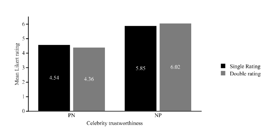
118
as compared to the single rating condition. This pattern of result provides a direct
replication of a previous study described earlier (White et al., 2014b) which focused on
affective (emotional) evaluations instead of trustworthiness ratings. The pattern of
results of both studies is contrasted in Figure 12 and Figure 13. In addition, we
reanalysed the results of (White et al., 2014b) in a Bayesian framework. The resulting
Bayes Factors and their interpretation can be found in Appendix A9.
Figure 12. Trustworthiness ratings as a function of experimental condition (White et al.,
2015).
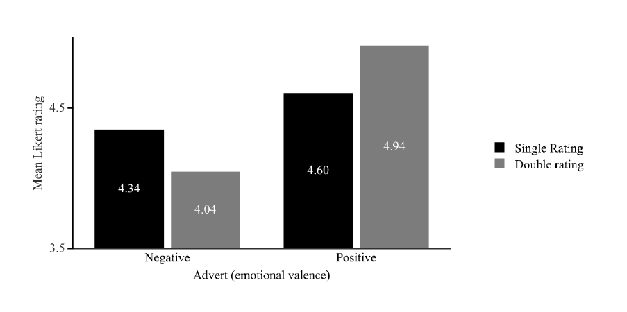
119
Figure 13. Emotional valence as a function of experimental condition (White et al.,
2014b).
White et al., (2014, 2015) argued that a model based on the axiomatic principles of QP
provides a viable and parsimonious, yet powerful explanation for these empirical
results. In quantum mechanics, it is a firmly established principle that the mere act of
taking a measurement changes the state of the system under investigation. The act of
taking a measurement is assumed to collapse Ψ, thereby converting and indeterminate
stochastic state (described by Schrödinger’s wave-function) into a discrete and precisely
determinable state. That is, the measurement constructs the state of the system due to
the collapse of the wave-function. In the context of cognitive processes, this means that
every judgment and decision can be regarded as an introspective measurement which
constructs the cognitive state (i.e., the state of the system under investigation) “on the
fly”. This change in the cognitive state (caused by a constructive introspective
measurement) has influences on subsequent measurements. This notion is clearly
opposed to classical (Markov) models which assume that the system is always in a
discrete state and that measurement (introspection) merely “reads out” an already pre-
120
existing state. Thus, the quantum perspective assumes that states are constructed
whereas the classical approach assumes that measurement are objective representations
of pre-existing states. In this context, the importance of stimulus-incompatibility should
be underscored. Stimulus-incompatibility is necessary criterion for the applicability of
the quantum probability framework to physical and psychological observables.
Incompatibility gives rise to the “no information without disturbance” maxim
(Heinosaari, Miyadera, & Ziman, 2015) and it is crucial factor for the emergence of
noncommutativity effects.
Taken together, the discussed experiments provide corroborating evidence for the
validity of the quantum cognition framework in respect to attitudinal and emotional
judgments.
Specifically, the results corroborate the importance of the quantum mechanical
noncommutativity principle. As discussed in the preceding paragraphs, a fundamental
difference between classical (Boolean) observables and quantum mechanical
observables is the dependence of sequential measurement outcomes on the specific
order in which measurements of quantum mechanical observables are performed.
Observables corresponding to noncommutative operators are called incompatible and
his asymmetrical inequality can be symbolically expresses as follows: AB BA 0.
The goal of our experimentation was to investigate this effect in the domain of
perceptual processes, i.e., in a rigorously controlled reductionistic psychophysics
framework. This approach has several advantages of the experiments conducted by
White et al., (2015, 2016). From a methodological point of view, visual stimuli can be
experimentally controlled in a much more precise way than, for instance, attitudinal or
emotional judgments, thereby reducing between-subject reliability. Furthermore, from a
phylogenetic perspective, the visual system is a much more basic system than the
121
emotional system and its anatomical and functional characteristics are shared with many
non-human species. If noncommutativity applies to human perception, one might
predict that it can also be observed in non-human species (e.g., primates, rodents, etc.).
In addition, our scientific knowledge of the visual system is much more sophisticated
compared to higher-order cognitive processes which are much more elusive. Therefore,
a reductionist approach would try to demonstrate noncommutativity at the lowest level
possible in order to establish a firm empirical foundation. Subsequently, the
generalisability of the phenomenon should be tested in more complex cognitive
situations. Our experimental approach can thus be regarded as an attempt to establish
noncommutativity in low-level perceptual processes in order to establish a
psychophysical foundation.
1.16 Current empirical research
The main question that motivated the present investigations is the following: What
exactly happens when people make perceptual decisions under conditions of
uncertainty? We were particularly interested in sequential noncommutativity effects and
the constructive role of introspective psychophysical measurements. Our theorising was
motivated by various psychophysical theories of complementarity (J. C. Baird, 1997).
Specifically, we wanted to investigate if the mere act of taking a psychophysical
measurement per se constructs the perceptual process in question. Random walk models
(e.g., Ratcliff & Smith, 2004; Usher & McClelland, 2001) which focus on reaction
times in various decision scenarios assume that evidence (information) is accumulated
over time until a specific decision-threshold is reached (cf. Harris, Waddington,
Biscione, & Manzi, 2014). In this class of “rise-to-threshold models”, the weight
associated with each option increases chronologically in a progressive manner.

122
However, at each discrete point in the temporal sequence the system is assumed to be in
a definite determinate state. This state can in principle be accessed by taking a
measurement. Moreover, it is assumed that the act of measuring does not influence the
state under investigation.
That is, classical models presuppose that a given system is consistently in a specific
state, even though the observers’ cognition of this state might be uncertain (e.g., a
hidden variable). This appears to be a very logical postulate. How else could one build a
model of a system if it is not in a definite (stable) and objectively measurable state at
any point in time?
However, this mainly unquestioned assumption stands in sharp contrast with one of the
main ideas of quantum probability (QP) which provides the axiomatic basis of quantum
theory. A fundamental insight derived from quantum theory is that taking a “physical
measurement” of a “physical system” actively creates rather than passively records the
property under investigation.
89
By contrast, classical theories assume that taking a
measurement merely reads out an already pre-existing state of a system. Moreover, QP
is incompatible with the classical notion that a given system (be it physical or
psychological) is always in a determinable state at any point in time. By contrast, QP
allows for the possibility that a system can be in a superpositional state in which n
possibilities can exist simultaneously. It is only when a measurement is taken that these
undetermined potentialities collapse into determinate actualities. In our experiment, we
tested various hypotheses which were a priori derived from the quantum probability
framework. We were particularly interested in noncommutativity in perceptual
89
In the context of decision-making, quantum cognition replaces the term “physical measurement” with
“human decision” and “physical system” with “cognitive system”.
123
processes and the constructive role of psychophysical measurements. Our predictions
are compatible with the results of previous research which investigated the same
phenomena in emotional and attitudinal judgments (White et al., 2015, 2014b).
124
CHAPTER 2. EXPERIMENT #1:
NONCOMMUTATIVITY IN SEQUENTIAL
VISUAL PERCEPTUAL JUDGMENTS
2.1 Experimental purpose
The primary objective of this experiment was to investigate noncommutativity in
sequential psychophysical measurements from a QP perspective, as has been previously
proposed by Atmanspacher & Römer (Atmanspacher & Römer, 2012), inter alia. QP
makes a priori and parameter-free predictions about sequential order effects (Z. Wang
et al., 2014). Specifically, our hypotheses were logically derived from the QQ-equality
principle (Z. Wang et al., 2014) discussed in the introduction. Thus, the present
experiment can be regarded as a translation of empirical findings from the
affective/emotional domain to the psychophysical domain.
Another interesting aspect which connects our research with previous pertinent
experiments (i.e., White et al., 2015, 2014b) is based on various embodied cognition
hypotheses concerning the affective properties of psychophysical stimuli. For instance,
it has been demonstrated that brightness is associated with positive emotional valence
and affect (B. P. Meier, Robinson, & Clore, 2004). Furthermore, virtuous attributes like
trustworthiness, morality, and ethical behaviour have been repeatedly linked to
brightness (e.g., Chiou & Cheng, 2013). From a cognitive linguistics point of view
(especially in the framework of conceptual metaphor theory (Lakoff, 1993; Lakoff &
Johnson, 1980)), the psychophysical stimuli we utilised can thus be regarded as
conceptually related to the stimuli which were utilised in related research (White et al.,
2015, 2014b). Specifically, stimulus brightness is conceptually closely associated with
cognitive representations of trustworthiness and positive affect (B. P. Meier, Robinson,

125
Crawford, & Ahlvers, 2007). That is, the neuronal sensorimotor grounding of affective
cognitive states (an abstract “intangible” concept) is based on concrete perceptual
properties (i.e., visual, tactile, auditory, olfactory, etc.). The nonconcrete concept
(affect) is mapped on the concrete domain (e.g., via Hebbian learning/synaptic long-
term potentiation).
90
For instance, it has been experimentally demonstrated that
brightness differences influence the evaluation of affective pictures (Lakens,
Fockenberg, Lemmens, Ham, & Midden, 2013), a research finding which emphasises
the general conceptual relation between more basic sensorimotor experiences (in the
Piagetian sense) and higher-order cognitive/affective constructs like attitudes and affect
(Dael, Perseguers, Marchand, Antonietti, & Mohr, 2016). Therefore, our experiment can
be interpreted from an embodied cognition point of view (Kurt, Eroğlu, Bayram
Kuzgun, & Güntekin, 2017). Specifically, brightness can be regarded as a source
domain and trustworthiness as the target domain. That is, the psychophysical domain is
more primary and provides the sensorimotor “primitives” (primary metaphors) for more
complex higher-order cognitive constructs (e.g., affect). However, for reasons of
parsimony and focus, a more detailed discussion of the associated cognitive
representations (embodied image schemata (Lakoff, 1987, 1993, 1994)) goes beyond
the scope of this chapter. For now, it is sufficient to note that “brightness” and “affect”
are neuronally and conceptually closely interlinked from an embodied cognition point
of view (Lakoff & Johnson, 1980; Lakoff & Nuñez, 2000). From a neuroscientific point
of view, there is thus significant neuronal overlap between the neural correlates of
representations of brightness and affect. ´Based on this theoretical background one
might therefore predict that noncommutativity effects observed in higher-order concepts
90
A more detailed description of embodied cognition and conceptual metaphor theory can be found
inAppendix B1. In the context of the current investigation, the representational association between
brightness perception and attitudinal/affective judgments (White et al., 2015, 2014b) is of particular
theoretical interest. We an overview of pertinent studies to undergird this claim.

126
like affect and trustworthiness (White et al., 2015, 2014b) generalise to the associated
embodiments of the concept, i.e., brightness perception.
In order to test our hypotheses, we utilised various parametric and non-parametric
inferential statistical testing procedures. This was done in order to increase the
robustness of our analyses and consequently the resulting logical inferences which are
based on these calculations. Moreover, statistics is currently in a process of reformation
(Cowles, 2014), especially in psychology, neuroscience, and the bio-medical sciences.
The “new statistics” are replacing the conventional Fisherian methods with more
“sophisticated” inferential techniques (Cumming, 2012, 2013, 2014; Eich, 2014).
91
In
the subsequent analyses, we utilised the most promising novel methodologies and
compared the results. By doing so we followed recent recommendation by the APA
journal “Psychological Science” which recently announced changes to its publication
guidelines. That is, we constructed confidence intervals and calculated effect-sizes for
all parameters of interest. Moreover, we went one step further and constructed
confidence interval for the effect sizes. In addition, we utilised the Vovk-Sellke
maximum p-ratio (VS-MPR) to convert conventional p-values into a more readily
interpretable format that is less prone to logical fallacies (Sellke, Bayarri, & Berger,
2001; Vovk, 1993). Furthermore, we applied bootstrapping techniques in order to check
the robustness of our results and to maximise inferential power. We obtained
bootstrapped confidence intervals for all parameters of interest. In addition, we
conducted our analyses in two complementary Bayesian frameworks in order to cross-
91
The suggested alternatives are mainly confidence intervals and effect sizes. However, these
recommendation do not address the crux of the problem, i.e., the logically inconsistent hybrid between
Fisherian and Neyman-Pearsonian methods (G Gigerenzer, 2004). A real-solution would advocate
genuine statistical thinking and reasoning (G Gigerenzer, 1998) and would promote context-dependent
analytical flexibility. It has been convincingly argued that Bayesian methods (particularly Bayesian
parameter estimation) are a viable alternative (Kruschke & Liddell, 2015, 2017c).
127
validate our analytical results and to gain additional information that is not available in
the frequentist framework. We performed a Bayes Factor analysis with appropriate
“prior robustness checks”. We also conducted a Bayesian bootstrap to compare results
with the previous frequentist bootstrap analysis. Moreover, we utilised Bayesian
parameter estimation via Markov chain Monte Carlo methods and tested our a prior
hypotheses using a HDI (high density interval) and ROPE (region of practical
equivalence) based decision algorithm. We were thus able to equate results from three
different statistical/methodological perspectives (viz., analytic triangulation), thereby
enabling convergent validation (Fielding, 2012).
2.2 A priori hypotheses
Our hypotheses were formulated a priori and they were derived from the pertinent
quantum cognition literature (Atmanspacher, 2014a, 2016; Atmanspacher & Römer,
2012; Z. Wang et al., 2013). We specifically focused on sequential noncommutative
effects in introspective visual judgments.
The directional (one-tailed) a priori hypotheses of primary interest were:
H
1
: Measuring the luminance of high luminance stimuli first results in a decrease in the
subsequent judgment for the low luminance stimuli as compared to the reverse order.
H
2
: Measuring the luminance of low luminance stimuli first results in an increase in the
subsequent judgment relative to reverse order.
In symbolic form expressed as follows:
H
A
: AB ≠ BA
where

128
A = high luminance visual stimuli
B
= low luminance visual stimuli
Note that H
A
can be expressed as a directional hypothesis (i.e., one-sided) by replacing
“≠” with either “<” or “>”.
2.3 Method
2.3.1 Participants and Design
The experiment was conducted in the psychology laboratory of the University of
Plymouth (United Kingdom) and ethical approval was obtained from the universities
human research ethics committee.
Eighty-two students from the University of Plymouth participated in this study (51
women and 31 men, ages ranging between 18 and 31 years, M
age
= 21.73; SD
age
= 4.17).
Students were recruited via a cloud-based participant management software (Sona
Experiment Management System®, Ltd., Tallinn, Estonia; http://www.sona-
systems.com) which is hosted on the universities webserver. In addition, a custom-made
website was designed in HTML, CSS, JavaScript, and “Adobe® Shockwave Flash -
ActionScript 2.0” (Yam, 2006) to advertise the study in an attractive way to the student
population (URL: http://irrational-decisions.com/sona/qp.html; see Appendix B2 for the
source-code). Participants received either course credit or a payment of £8 for their
participation.

129
2.3.2 Apparatus and materials
In order to support the open-source philosophy (Vainio & Vaden, 2012) and to facilitate
replicability and the “openness of science” (Boulton et al., 2012) we used open-source
software whenever this was feasible and uploaded all materials and the resulting dataset
on our webserver at http://irrational-decisions.com/qp-exp1/.
92
For the visual decision-making task, two singleton grey rectangles (dimensionality: 220
x 220px) with two different luminance levels were created using the open-source raster
graphics editor GIMP (http://git.gnome.org/browse/gimp; see Peck, 2006). We utilised
“Fechnerian scaling” (Dzhafarov, 2002; Dzhafarov & Colonius, 2001, 2005) for the
design of the psychophysical stimuli, a psychophysical scaling technique which has also
been implemented in the “Fechner” R package (Ünlü, Kiefer, & Dzhafarov, 2009).
To systematically control stimulus luminance levels, we varied the V-parameter of the
92
We are convinced that transparency should be one of the hallmarks of proper scientific research and
nowadays there is no excuse why one should not make all material/data publicly available. Nowadays
researchers can easily include a URL in all their publications or use the Open Science Framework (Foster,
MSLS & Deardorff, MLIS, 2017), or similar repositories in order to foster “open knowledge” and “open
data” (Boulton et al., 2012; Molloy, 2011). This would facilitate replication and, consequently, enhance
the reliability of scientific findings. In addition it has been cogently argued that “open science is a
research accelerator” (Woelfle, Olliaro, & Todd, 2011). The “replication crisis” is currently of great
concern (Aarts et al., 2015; Baker, 2016; Munafò et al., 2017; Peng, 2015). A conscience discussion of
this multifaceted “metascientific” topic is provided in a recent N
ATURE article (Schooler, 2014).
Furthermore, this approach would enable other researchers to evaluate the validity of the reported
findings by reanalysing the data (third party verification). Unbiased independent researchers who do not
have any “unconscious” theory-driven vested interests (i.e., no confirmation bias) might discover patterns
in the data which escaped the author’s attention and they might be able to test novel hypotheses which
were not part of the initial research agenda. Science should be a collective endeavour and ego-
involvement should be minimized while knowledge accumulation should
be the primary motif.
Collectively, society would benefit from a more transparent approach towards science, especially in the
long run. Moreover, openly publishing data could facilitate (possibly AI/machine learning driven) meta-
analytic research (e.g., large-scale data mining). Such (semi-)automated procedures have the potential to
significantly speed up general scientific progress. Furthermore, publishing negative results could
potentially alleviate the long-standing and hitherto unresolved problem of α-error inflation (for more
information on this crucial topic see http://irrational-decisions.com/?page_id=520
)

130
HSV colour gamut (see Figure 14). The HSV colour model was created by Alvy Ray
Smith in 1978 for computer graphics applications. HSV is an acronym for “hue,
saturation, and value”, and is also often abbreviated with HSB (B for brightness).
We chose the HSV model due to its geometric properties
93
and because previous
experimental research showed that it displays reliable perceptual properties (Schwarz, et
al., 1987). Furthermore, the HSV gamut allows for geometric (and
symmetric/isomorphic) transformations which could be mapped onto projection vectors
in the QP model in order to establish accompanying correlation coefficients. We created
an interactive web-based example of the HSV model using “Adobe® Shockwave Flash
- ActionScript 2.0” (Yam, 2006). The application can be accessed under the following
URL:
http://irrational-decisions.com/?page_id=875
For the experimental stimuli, we applied the following parametrization to the V-value:
• High luminance stimuli: HSV: 0,0,60. (RGB: 153,153,153)
• Low luminance stimuli: HSV: 0,0,40. (RGB: 102,102,102)
The resulting visual stimuli can be downloaded from the following URLs as *.jpg files:
http://irrational-decisions.com/phd-thesis/visual-stimuli/low-luminance.jpg
http://irrational-decisions.com/phd-thesis/visual-stimuli/high-luminance.jpg
93
The notion of subspaces of a Hilbert space is a geometrical one and quantum probability is oftentimes
referred to as “projective probability” (Brody & Hughston, 2001; Busemeyer & Bruza, 2012; Z. Wang et
al., 2013). Consequently, geometric colour spaces lend themselves as good candidates for exact
quantitative modelling in future psychophysics experiments. Experimental results could then be
correlated to the geometric quantum probability model by a talented mathematician/geometrician.

131
Figure 14. The HSV colour space lends itself to geometric modelling of perceptual
probabilities in the QP framework.
94
2.3.3 Experimental application in PsychoPy
The experiment was implemented in PsychoPy (J. W. Peirce, 2007, 2008) which is
based on Python (Python Software Foundation, 2013). PsychoPy
95
is an open-source
application for the design, programming, and presentation of experimental protocols
with applicability to a broad array of neuroscience, psychology, and particularly
psychophysics research. Although the stimuli timing functionality is a matter of
ongoing debate, PsychoPy can achieve high levels of accuracy and precision with
regards to the presentation of brief and quickly alternating visual stimuli (Garaizar &
Vadillo, 2014). A detailed benchmark report can be found in Appendix B3. The
94
It should be noted that the HSV model has several shortcomings. According to scientific nomenclature,
lightness is defined as the perceived quantity of emitted light (and not emitted light itself as objectively
measured). The HWB (Hue-Whiteness-Blackness) model has been suggested as an alternative based on a
more intuitive mental model of colour space (Lou, Cui, & Li, 2006; A. R. Smith & Lyons, 1996). The
conversion of HSV to HWB is as follows:
H → H
W → (1 - S) V
B → 1 - V
95
PsychoPy is a powerful viable alternative to proprietary software-packages like or E-Prime™ or
Presentation™. Given that PsychoPy is entirely coded in Python (which can be utilised as a free
alternative to Matlab™ (Blais, 2007; Jurica, 2009; Millman & Aivazis, 2011)), its capabilities can be
extended with countless Python modules, packages, and libraries.

133
2.3.4 Experimental Design
The basic structure of the experiment was a factorial repeated measures design in which
the presentation order of two singleton visual stimuli with different luminance levels
was randomly alternated in order to investigate noncommutative sequential effects in
visual judgments (Bradley, 1958). We utilised a fully counterbalanced Latin-square
design (Gaito, 1958; Grant, 1948). The experimental conditions were thus as follows:
V
00
= low luminance → low luminance
V
01
= low luminance → high luminance
V
11
= high luminance → high luminance
V
10
= high luminance → low luminance
The dependent variable was the condition dependent brightness rating which was
recorded on a visual analogue scale as described in the ensuing subsection.
2.3.5 Procedure
Before the commencement of the study, participants were briefed (see Appendix B4)
and accorded written informed consent (see Appendix B5). Subsequently, participants
were seated in front of a personal computer (a detailed PC/graphic-card configuration
report can be found in Appendix B3) and received further instructions.
2.3.6 Sequential visual perception paradigm
First, we collected general demographic information. Participants completed the form
depicted in Figure 15.

134
Figure 15. Demographic data collected at the beginning of the experiment.
After mouse clicking the “OK” button, the practice-phase of the visual perception
paradigm was initiated. Participants were informed that they would perform a test of
visual acuity which involved the perception of minute luminance differences.
Participants were presented with a set of instructions (for verbatim transcript
seeAppendix B6). Participants were required to judge the perceived brightness of a
series of grey rectangles on a computerized visual analogue scale (Aitken, 1969),
henceforth acronymized as VAS. The polar dimensionality of the VAS ranged from
“not bright” to “very bright” (see Appendix B6 for screenshots). The respective VAS
coordinates were automatically converted by PsychoPy into numerical values ranging
from 1-10. We opted for a VAS because it allows for a more fine-grained continuous
measure as compared to the widely employed discrete Likert scale (Likert, 1932);
thereby increasing statistical sensitivity (i.e., discriminatory power) in the subsequent
statistical analysis (for a direct comparison of both measurment apporaches see Van
Laerhoven, Van Der Zaag-Loonen, & Derkx, 2004). An additional advantage of visual
analogue scales over numerical rating scales is that the interval between values is not
only interpretable as an ordinal measurement but also as an interval and ratio-type
measurement (for an extended discussion see Price, Staud, & Robinson, 2012). It can
thus be concluded that visual analogue scales have superior psychometric properties
compared to their numerical counterparts. In PsychoPy, we fixed the precision

135
parameter of the VAS to 100, i.e., each increment was subdivided into 1/100
th
of a tick-
mark. This configuration enabled an extremely fine-grained measurement of responses.
After each stimulus presentation, the VAS marker was by default automatically reset to
the absolute midpoint of the scale. Before the commencement of the experimental trials,
participants completed a practice block consisting of 4 trials. During the practice phase,
participants were acquainted with the workings of the VAS and the general
experimental procedure.
After that, the experimental block was automatically initiated. An experimental trial
consisted of the presentation of a singleton grey rectangle which either displayed high
luminance or low luminance. Stimulus presentation order was randomised within
PsychoPy. In 50% of the trials participants had to judge the brightness of low luminance
stimuli and in the remaining trials they were required to judge the brightness of high
luminance stimuli. Stimuli were either preceded by stimuli of equivalent luminance
(e.g., high luminance followed by high luminance) or by stimuli with different
luminance levels (e.g., low luminance followed by high luminance). Each stimulus was
presented for 60 frames (≈ 1000.2ms).
96
After a manual response was emitted (single
left mouse click on the VAS), the next trial was automatically initiated (starting again
with the visual fixation of the crosshair). In sum, the task of participants was to evaluate
the visual stimuli which were presented in a randomly varying sequential order. In the
PsychoPy backend, trials were programmatically organised in a loop. Randomization
was archived by utilising the Python "NumPy" package (Van Der Walt, Colbert, &
96
Vertical refresh rate of screen = 60Hz
1 frame = 1000ms/60 ≈ 16.67ms (frame to frame variability on average = 2.18ms)
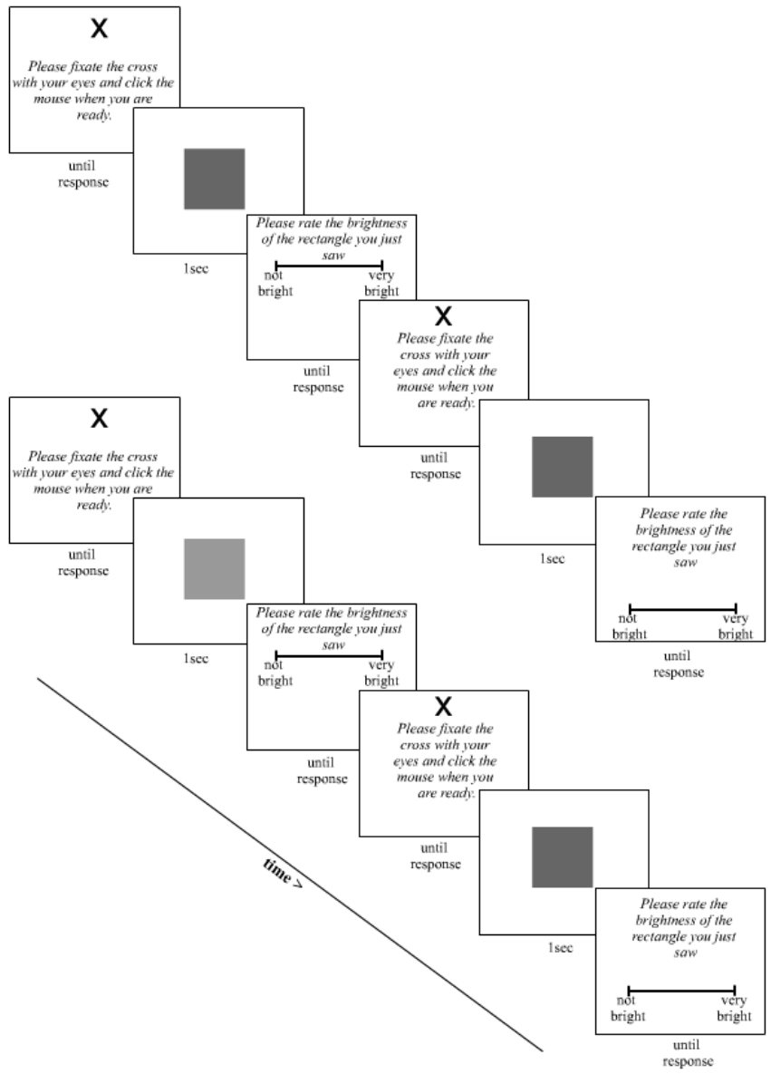
137
The within-trial sequence of events was as follows: Initially, a white fixation cross
(crosshair) was displayed on a black background until a manual response (single left
mouse-click) was emitted. The following instructions were presented to participants:
“Please fixate the cross with your eyes and click the mouse when you are ready”. Next,
a rectangle of either high or low luminance appeared in the centre of the screen (screen
size = 1920 x 1080, the application was executed in fullscreen mode) with a fixed
duration of 60 frames. The rectangle was then replaced by a VAS rating request which
was presented until a response was emitted. After that, the next rectangle appeared for
the same temporal duration followed by the final rating request. In sum, each participant
completed a total of 600 experimental trials. Upon completion of the experiment,
participants were debriefed (see Appendix B7) and were given the possibility to ask
questions concerning the purpose and theoretical background of the study. Finally,
participants were thanked for their cognitive efforts and released.
2.3.7 Statistical Analysis
In order to test the formulated hypotheses, we utilised various parametric and non-
parametric inferential statistical testing procedures. This was done in order to increase
the robustness of our analyses and consequently the resulting logical inferences which
are based on these calculations. Moreover, statistics is currently in a process of
reformation (Cowles, 2014), especially in psychology and neuroscience. The “new
statistics” are recommended by the APA and they are extending conventional Fisherian
NHST with slightly more sophisticated inferential techniques (Cumming, 2012, 2013,
2014; Eich, 2014). Currently, classical NHST is unfortunately still the most dominant
inferential approach in psychology and the bio-medial sciences (by a very large margin)
and the APA recommendations do not really address the core of the issue which is the

138
incompatible hybrid of Fishery and Neyman-Pearsonian methods. The vast majority of
researchers exclusively utilise NHST in their analyses, despite the fact that NHST has
been severely criticised on logical grounds (Cohen, 1995). The underlying syllogistic
logic is widely misunderstood by the majority of professional researchers who are
teaching their misinterpretations to students (Haller & Krauss, 2002), thereby
perpetuating the delusional NHST meme. Consequently, logical conclusion based on
NHST are frequently fallacious and invalid
97
. The consequences for the progress of
science are obviously far reaching. We conducted a survey amongst researchers within
the CogNovo programme and found that 17 out of 18 participants (professors, doctors
and PhD students) were unable to interpret a simple independent samples t-test (see
Appendix A8 for a synopsis of the survey). The results are representative of the larger
population and have been replicated in various countries i.e., Germany, UK, USA (G
Gigerenzer, 2004; Haller & Krauss, 2002). More than 80% of professional researchers
who teach statistics at universities to students commit significant logical fallacies when
asked to interpret a simple independent-samples t-test. The most common fallacy is the
replication fallacy which fallaciously assumes that the p-value conveys information
about the replicability of a given finding. Current statistical practices have been
appropriately described as “mindless social rituals” by experts in the field of decision-
making (G Gigerenzer, 1993, 2004; G Gigerenzer & Krauss, 2004). We are convinced
that every scientist should ponder the logic of hypothesis testing because it lies at the
very heart of the scientific endeavour. Critical thinking (instead of blind conformity to
social norms) is of great importance for every serious researcher. It has been forcefully
argued that “psychologists must change the way they analyse their data” in order to
97
We discussed the “pitfalls of null hypothesis testing” extensively in a workshop and we also collected
empirical data on the ubiquitous misinterpretation of p-values (see). The associated video is available
under the following URL: http://www.cmharris.co.uk/?page_id=1444
139
improve the scientific discipline (Loftus, 1996; E. J. Wagenmakers, Wetzels,
Borsboom, & Maas, 2011; E. J. Wagenmakers, Wetzels, Borsboom, & van der Maas,
2011) and we followed these sensible recommendations by utilising various
nonconventional approaches.
In the subsequent analyses, we utilised the most promising “novel” statistical
methodologies. We followed recent recommendation by the APA flagship journal
“Psychological Science” which recently announced changes to its publication
guidelines. We constructed confidence intervals and calculated effect-sizes for all
parameters of interest. Moreover, we went one step further and constructed confidence
interval for the effect sizes. We also went beyond the somewhat superficial
recommendations and utilised the Vovk-Sellke maximum p-ratio (VS-MPR) to convert
conventional p-values into a more readily interpretable format that is less prone to
logical fallacies (Sellke et al., 2001; Vovk, 1993). Furthermore, we used bootstrapping
techniques in order to check the robustness of our results and to maximise inferential
power. We obtained bootstrapped confidence intervals for all parameters of interest. In
addition to NHST, we conducted our analyses in different Bayesian frameworks in
order to cross-validate our analytical results. We performed a Bayes Factor analysis
with appropriate “prior robustness checks” and we computed a “Bayesian bootstrap” to
compare results with the previous frequentist nonparametric bootstrap analysis.
Moreover, we performed Bayesian parameter estimation using Markov chain Monte
Carlo methods and tested our a priori hypotheses using a HDI (high density interval)
and ROPE (region of practical equivalence) based decision-algorithm (Kruschke, 2014).
We were thus able to equate results from various statistical paradigms (statistical
triangulation), thereby increasing the verisimilitude of our inductive inferences (Festa,
1993).

140
2.3.8 Data treatment and statistical software
The PsychoPy-output was stored in comma-separated value files (*.csv files) which
were merged into a single file. Each file included an anonymized participant ID, the
date, and the starting time of the experiment, the demographic data, and the
experimental data. Statistical analysis was primarily conducted by utilizing the open
source software R v3.3.2 (R Core Team, 2013) and we extended its capabilities with the
open-source RStudio IDE
98
v1.1.383 (RStudio Team, 2016). Moreover, we imported
the “ggplot” library (Wickham, 2009, 2011) for plotting data. Furthermore, we
utilised “knitR” v1.17 (Y. Xie, 2014, 2015) and “Pandoc” v2.0.0.1 (Krewinkel &
Winkler, 2016; Krijnen, Swierstra, & Viera, 2014; Tenen & Wythoff, 2014) for
automated dynamic document creation and conversion.
2.3.9 Frequentist NHST analysis
First, we computed various diagnostics (Table 1) and investigated the distributional
characteristics of the data. In order to examine whether the data was normally
distributed and to check for spurious outliers we utilised various visualisation
techniques. We created Q-Q plots for all conditions (see Appendix B8) and median-
based boxplots (Appendix B12). In addition, we visualised the data as using the
“beanplot” package in R (Kampstra, 2008) (see Figure 17). Beanplots are a novel
and creative way to visualise data (Juutilainen, Tamminen, & Röning, 2015). They
provide much more detailed statistical/distributional information than conventional
boxplots and line-graphs. Boxplots and related conventional visualisation techniques are
regularly utilised to compare univariate data (Frigge, Hoaglin, & Iglewicz, 1989).
98
IDE is an acronym for “Integrated Development Environment”.

141
However, a significant disadvantage of classical boxplots is that they fail to display
crucial distributional information. Moreover, they are not readily interpretable by non-
mathematician (Kampstra, 2008). Beanplots are a viable alternative for visual
comparison of univariate data between experimental conditions. Individual observations
are displayed as small horizontal lines in a one-dimensional scatter plot. In addition, the
estimated density of the distributions is displayed (we chose a Gaussian kernel) and the
average is demarcated by a thick horizontal black line. Thusly, beanplots facilitate
comparisons between experimental conditions and they enable the analyst to evaluate if
the dataset contains sufficient observations to render the difference between
experimental conditions meaningful from a statistical point of view. Furthermore,
anomalies in the data (e.g., skewness, kurtosis, outliers, duplicate measurements, etc.)
are readily identifiable in a beanplots (Kampstra, 2008). For purposes of direct between-
group comparison, the associated R package provides the option to create a special
asymmetric beanplot. We made use of this inherent function and created asymmetric
beanplots which directly contrast the distributional characteristics of the pertinent
experimental conditions (see Figure 18).
Table 1
Descriptive statistics for experimental conditions.
N
Mean
SD
SE
v00
82
3.290
1.010
0.112
v10
82
3.710
0.930
0.103
v01
82
7.220
1.130
0.125
v11
82
6.690
1.070
0.118

142
2.3.10 Assumption Checks
Visual inspection of Q-Q plots (see Appendix B8) indicated that the Gaussianity
assumption is satisfied, and that parametric hypothesis testing is appropriate for the data
at hand (Wilk & Gnanadesikan, 1968). We utilised the R package “moments”
99
to
evaluate skewness
100
and kurtosis
101
of the sample distributions. The indices of both
distributional characteristics where within the ordinary range of ±2 and ±7, respectively
(cf. Cain, Zhang, & Yuan, 2016; Groeneveld & Meeden, 1984), indicating that the data
is neither saliently skewed nor overtly kurtic. We also performed formal p-value based
significance tests of skewness and kurtosis, i.e., D’Agostino’s K
2
skewness test
(D’Agostino, 1970) and the Anscombe-Glynn kurtosis test (Anscombe & Glynn, 1983),
both of which supported the stipulated Gaussianity assumption for all variables.
Moreover, we computed the “Probability Plot Correlation Coefficient” (Filliben, 1975)
for each experimental condition using the “PPCC”
102
package in R. The PPCC tests
were performed with 10000 Monte Carlo simulations. The outcome of all four PPCC
tests confirmed distributional Gaussianity (see Appendix B18). In addition, we tested
for heteroscedasticity (i.e., σ
1
2
≠ σ
2
2
) which is associated with the extensively studied
Behrens-Fisher problem which may cause an inflated α-level (Sawilowsky, 2002).
99
https://cran.r-project.org/web/packages/moments/moments.pdf
100
The associated formula for the Fisher-Pearson coefficient of skewness is:
(
)
/
, where signifies the mean, s the standard deviation, and N the number of data points.
101
The definition of Pearson’s measure of kurtosis is:
(
)
/
, where signifies the mean, s the standard deviation, and N the number of data points.
102
Available on CRAN: https://cran.r-project.org/web/packages/ppcc/ppcc.pdf

143
However, the ratio of variances confirmed homoscedasticity, i.e., the results of the F-
test confirmed homogeneity of variances.
103
103
It is a common strategy to test for heteroscedasticity prior to a t-test. If the F-test on homogeneity of
variances is statistically nonsignificant, the researcher continues with the parametric t-test. Otherwise
alternative procedures (e.g., Welch-Aspin) which modify the degrees of freedom a required. However,
this approach (i.e., making the t-test conditional on the F-test) can lead to an inflation of experiment-wise
α-errors. That is, the sequential nature of protected testing automatically effects the nominal α-level.
Moreover, it has been reported that a F-test protected t-test can lead to a significant loss in statistical
power under Gaussianity (Sawilowsky, 2002). We will discuss issues associated with multiple hypotheses
tests in more detail in the general discussion section in the context of α-inflation.
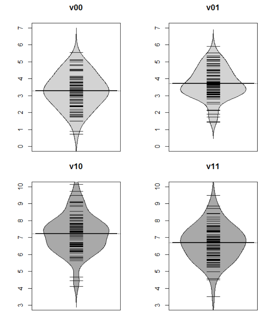
144
Figure 17. Beanplots visualising distributional characteristics of experimental
conditions.
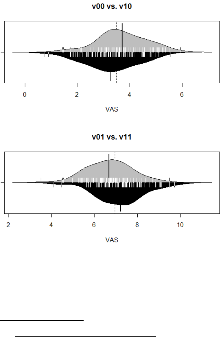
145
Note: The thin horizontal black lines represent individual data points and the thick
black line indicates the grand mean per condition. The shape of the bean visualises the
density of the distributions (Gaussian kernel).
Figure 18. Asymmetric beanplots visualising pairwise contrasts and various
distributional characteristics.
104
104
A high resolution (zoomable) vector graphic for closer inspection is available under the following
URL: http://irrational-decisions.com/phd-thesis/beanplots-exp1.pdf
The associated R syntax can be found under the following URL: http://irrational-
decisions.com/?page_id=2358

146
In order to investigate the distributional characteristics of the differences between
means, we performed the Shapiro-Wilk’s W test (S. S. Shapiro & Wilk, 1965). It has
been demonstrated in large scale Monte Carlo simulation experiments (Razali & Wah,
2011) that the Shapiro-Wilk’s W test
105
possess good characteristics (e.g., robustness,
statistical power) in comparison to other popular tests of Gaussianity (e.g.,
Kolmogorov-Smirnov test, Lilliefors test, Anderson-Darling test, Cramér-von Mises
test). The results reported in Table 2 suggest that Gaussianity can be assumed for the
differences between means (the reported values refer to the mean brightness judgments
to the second stimulus on each trial). Given that the normality assumption was satisfied
we proceeded to test our hypotheses in a parametric inferential framework.
106
Table 2
Shapiro-Wilk’s W test of Gaussianity.
W
p
v00
-
v10
0.975
0.112
v01
-
v11
0.986
0.533
Note. Significant results suggest a deviation from Gaussianity.
105
The associated formula is =
(
()
)
(
)
.
106
For the paired samples t-test, it is not important that the data is normally distributed per condition. The
t-test merely assumes that the differences in means are normally distributed (this is evaluated by utilising
W).

147
2.3.11 Parametric paired samples t-tests
In order to test our a priori formulated hypotheses
107
formally, we conducted two paired
samples “Student” t-tests (Gosset, 1908). The results of both pairwise comparisons
(two-tailed) were statistically significant at the conventional arbitrary α-level of 0.05 (R.
Fisher, 1956). The first t-test indicated that low luminance stimuli were on average rated
significantly lower in brightness when anteceded by equivalent stimuli (V
00
; M=3.29,
SD=0.93), as compared to low luminance stimuli anteceded by high luminance stimuli
(V
10
; M=3.71, SD=0.93), M
Δ
=-0.42; t(81)=-3.07, p=0.003, 95%CI [-0.69, -0.15];
Cohen’s d=-0.34,
108
95%CI
for d [-0.56, -0.12]. By contrast, the brightness of high
luminance stimuli was on average rated significantly higher when the high luminance
stimuli were anteceded by low luminance stimuli (V
01,
M=7.22, SD=1.13), relative to
high luminance stimuli anteceded by equivalent stimuli (V
11
, M=6.69, SD=1.07), M
Δ
=-
0.53; t(81)=-3.43, p<0.001, 95%CI [0.22, 0.83]; Cohen’s d=-0.38, 95%CI for d [-0.15, -
0.60]
109
. The effect was thus slightly more pronounced for the second orthogonal
contrast. In sum , the analysis corroborated our a priori hypotheses and confirmed the
predictions formulated by Atmanspacher & Römer (Atmanspacher & Römer, 2012).
Given that multiple comparisons were conducted, it was necessary to apply a correction
of α in order to prevent α-error inflation (i.e., the experimentwise error which has an
identifiable maximum). We applied a classical single-step Bonferroni correction (O. J.
Dunn, 1958, 1961) and adjusted the α-level accordingly.
110
Both comparisons remained
107
That is, the noncommutativity hypotheses AB ≠ BA described in section 2.2.
108
Effect sizes were calculated based on the formula described by Moors (R. Fisher, 1956):
=
where the pooled standard deviation (s) is defined as =
(
)
(
)
109
Given the widespread misinterpretation of conventional confidence intervals (Hoekstra et al., 2014) we
provide additional tolerance intervals (Krishnamoorthy & Mathew, 2008) based on the Howe method
(Howe, 1969) inAppendix B13.
110
We utilised a classical single-step Bonferroni correction according to the following formula:

148
statistically significant at the conventional/normative level. However, given that we has
directional a priori hypotheses and given that we only reported two-sided tests (in order
to prevent controversies), it could be argued that the Bonferroni correction was
unnecessary because the possible inflation of α was counterbalanced by the
bidirectionality of the two hypotheses testing procedures, given that = 2
(
>
|
|)
, where T is the critical value of the Student distribution. However, the topic
of α-inflation is of great importance for logically valid scientific inferences, but it is
largely neglected by researchers
111
. We will discuss widespread issues associated with
multiple comparison adjustments (i.e., experimentwise and familywise error rates) in
greater detail in section 6.11.5.
In addition to the conventional parametric t-test, we computed the Wilcoxon signed-
rank test (Wilcoxon, 1945) which provides a powerful nonparametric alternative to the
t-test.
112
The Wilcoxon test computes the test statistic W and the corresponding p-value.
It is a test of the null hypothesis (at the nominal α-level) that the distribution of the data
is symmetric around a prespecified median value μ (i.e., μ = 0).
113
In the current
analysis, W is utilised to test if the difference of the paired observations is centred
symmetrically around μ = 0. For larger samples (>50) the test is based on a Gaussian
, where signifies the total number of hypotheses tested.
Specifically, the Bonferroni procedure stipulates that H
1
should be rejected if
where
is the
arbitrarily/idiosyncratically (Nuijten et al., 2016b) specified p-value for testing H
1
.
111
A meta-analysis of more than 30000 published articles indicated that less than 1% applied α-
corrections for multiple comparisons even though the median number of hypothesis tests per article was 9
(Conover, 1973; Derrick & White, 2017; Pratt, 1959).
112
Monte Carlo studies demonstrated that Wilcoxon test can be three to four times more powerful in
detecting differences between means when the Gaussianity assumption is not met (R. C. Blair & Higgins,
1985; R. Clifford Blair & Higgins, 1980). Given that less than 5% of datasets in psychology are
distributionally symmetric (Micceri, 1989), it has been argued that “the Wilcoxon procedure should be
the test of choice” (Sawilowsky, 2002, p. 464). Moreover, Sawilowsky emphasizes the importance of
habits which antagonise statistical innovation: “The t-test remains a popular test, however, most likely
due to the inertia of many generations of classically parametrically trained researchers who continue its
use for this situation” (Sawilowsky, 2002, p. 464).
113
A limitation of the Wilcoxon test is that equivalent pairs are discarded from the analysis. If this is of
particular concern, modified versions can be utilised (Charles, Jassi, Narayan, Sadat, & Fedorova, 2009).
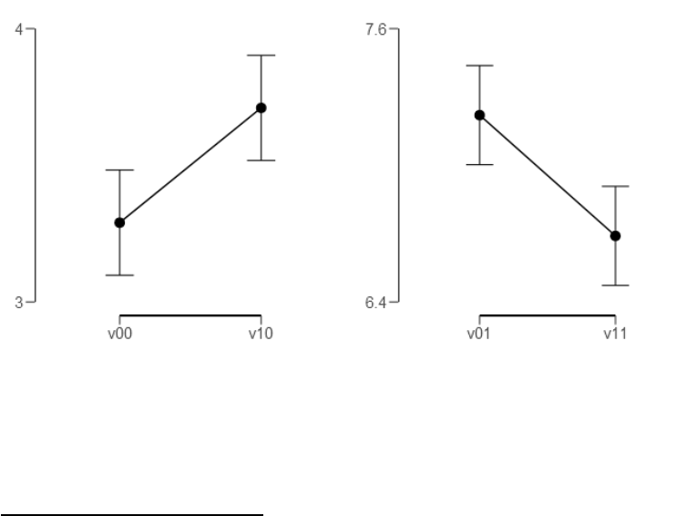
149
approximation to calculate p. However, the Wilcoxon signed-rank test can also be used
to compute exact statistics if the Boolean “exact” parameter is set to “TRUE” in R. In
our analysis, this parametrisation did not make any meaningful difference. Hence, we
only report the default test statistic. Moreover, the Hodges-Lehmann estimator
(Lehmann, 1998; Oja, 2010) was employed to calculate confidence intervals for the
nonparametric location parameter and the matched rank biserial correlation (Cureton,
1956; Woolson, 2008) was utilised to calculate nonparametric effect sizes
114
(with
associated 95% confidence intervals).
In résumé, the results of the Wilcoxon tests were in line with the conclusions derived
from the t-tests (even though the exact numerical values diverged). Both methods
(parametric vs. nonparametric) indicated statistically significant differences between
experimental conditions and confirmed our a priori predictions concerning
noncommutativity in visual perceptual judgments. The statistical results of both
analyses are summarised in Table 3 and a visual synopsis is provided in
Figure 19. “Connected boxplots” are available under the following URLs:
114
If exact p-values are available, an exact confidence interval is obtained by the algorithm described in
Bauer (1972).
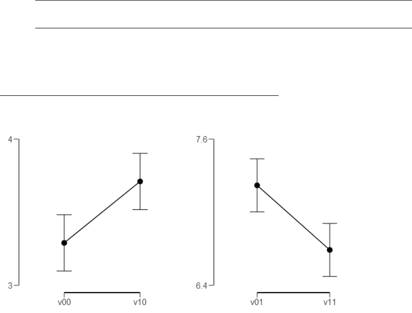
150
• http://irrational-decisions.com/phd-thesis/connected-boxplots-exp1-v00-v10.pdf
• http://irrational-decisions.com/phd-thesis/connected-boxplots-exp1-v01-v11.pdf
In addition, the complete results are summarised under the following URL:
http://irrational-decisions.com/phd-thesis/results-exp1.html
Figure 19. Statistically significant differences between grand means of experimental
conditions and their associated 95% confidence intervals.

151
Table 3
Paired samples t-tests and nonparametric Wilcoxon signed-rank tests
95% CI for Location
Parameter
95% CI for
Effect Size
Test
Statistic
df
p
VS-
MPR*
Location
Parameter
SE
Difference
Lower
Upper
Effect
Size
Lower
Upper
v00
-
v10
Student
-3.071
81
0.003
21.69
-0.420
0.137
-0.692
-0.148
-0.339
-0.561
-0.116
Wilcoxon
1089.000
0.005
14.69
-0.471
-0.714
-0.160
-0.360
-0.555
-0.127
v01
-
v11
Student
3.427
81
< .001
55.04
0.530
0.155
0.222
0.838
0.378
0.153
0.601
Wilcoxon
2442.000
< .001
79.89
0.544
0.239
0.838
0.435
0.214
0.614
* Vovk-Sellke Maximum p -Ratio: Based on the p -value, the maximum possible odds in favor of H over H equals 1/(-e p log( p ))
for p ≤ .37 (Sellke, Bayarri, & Berger, 2001).
Note. For the Student t-test, location parameter is given by mean difference d ; for the Wilcoxon test, effect size is given by the
Hodges-Lehmann estimate.
Note. For the Student t-test, effect size is given by Cohen's d ; for the Wilcoxon test, effect size is given by the matched rank biserial
correlation.

152
2.3.12 Bayes Factor analysis
In this section, we report a Bayes Factor analysis with robustness checks for various
priors and a sequential analysis for the evolution of the Bayes Factor as a function of
the number of participants (i.e., a time series of evidential flow). We conducted the
Bayes Factor analyses using the “BayesFactor” package (Richard D. Morey,
Rouder, & Jamil, 2014) in R. In addition, we utilised the open-source software JASP
115
which is based on the same R package. The dataset, the results, and the corresponding
JASP analysis script can be downloaded from the following URL to facilitate
“analytical reviews” as recommended by Sakaluk, Williams, & Biernat (2014):
http://irrational-decisions.com/phd-thesis/exp1.jasp.
116
At the conceptual meta level, the
primary difference between the frequentists and the Bayesian account is that the former
treats data as random and parameters as fixed and the latter regards data as fixed and
unknown parameters as random. Given the “cognitive context” (pertinent background
knowledge is lacking), and in order to keep the analysis as objective as possible
(objective Bayes
117
), we avoided opinionated priors and applied a noncommittal
115
JASP is currently dependent on more than 100 R packages. An up-to-date list of the included R
packages can be found under the following URL: https://jasp-stats.org/r-package-list/
116
This allows the interested reader to replicate the analysis with various idiosyncratic parametrisations,
e.g., in a “subjective Bayes” framework (Berger, 2006).
117
For more information on “objective Bayesianism” we refer the interested reader to a pertinent
publication by Berger (1977).

153
(diffuse) Cauchy prior
118
as advocated by Sir Harold Jeffreys (Jeffreys, 1939, 1946,
1952)
119
.
“The prior distribution is a key part of Bayesian inference and represents the
information about an uncertain parameter that is combined with the probability
distribution of new data to yield the posterior distribution, which in turn is used for
future inferences and decisions.” (Gelman, 2006, p. 1634)
Instead of using the standard Cauchy distribution that was Jeffreys’ default choice (r =
1), we set the scale parameter of the Cauchy distribution to 1/ √ 2 ≈ 0.707, the present
de facto standard in the field of psychology (Gronau, Ly, & Wagenmakers, 2017). We
fixed the location parameter for the effect size of the prior distribution under H
1
to δ =
0. It has been pointed out that Bayes factors with the Cauchy prior are slightly biased
towards H
0
(Rouder, Speckman, Sun, Morey, & Iverson, 2009), i.e., the Cauchy prior is
slightly conservative towards H
1
. The noninformative (noncommittal) parametrisation
of the Bayesian model we applied is as follows (“objective Bayes” (Berger, 2006)):
H
1
: δ Cauchy(0,r)
A Bayes Factor can range from 0 to ∞ and a value of 1 denotes equivalent support for
both competing hypotheses. Moreover, LogBF
10
can be expressed as a logarithm
118
In a seminal paper entitled “Inference, method, and decision: towards a Bayesian philosophy of
science” Rosenkrantz (Rosenkrantz, 1980, p. 485) discusses the Popperian concept of verisimilitude
(truthlikeness) w.r.t. Bayesian decision making and develops a persuasive cogent argument in favour of
diffuse priors (i.e., C-systems with a low λ). In a related publication he states: “If your prior is heavily
concentrated about the true value (which amounts to a 'lucky guess' in the absence of pertinent data), you
stand to be slightly closer to the truth after sampling than someone who adopts a diffuse prior, your
advantage dissipating rapidly with sample size. If, however, your initial estimate is in error, you will be
farther from the truth after sampling, and if the error is substantial, you will be much farther from the
truth. I can express this by saying that a diffuse prior is a better choice at 'almost all' values of [q1] or,
better, that it semi~dominates any highly peaked (or 'opinionated') prior. In practice, a diffuse prior never
does much worse than a peaked one and 'generally' does much better…” (1946)
119
Mathematically, Jeffreys’ prior is defined as follows: (
)
(
). It has the advantage that it is
scale invariant under various reparameterizations, for details see Jeffreys (e.g., G Gigerenzer & Hoffrage,
1995).

154
ranging from -∞ to ∞. A BF of 0 denotes equal support for H
0
and H
1
. Appendix B20
contains additional information on the Bayes Factor, the choice of priors, and various
advantages of Bayes Factor analysis over NHST.
For the first pairwise comparison we computed (experimental condition V
00
vs. V
10
), we
obtain a Bayes Factor of BF ≈ 9.12 indicating that the data are about 9 times more
likely under H
1
than under H
0
, i.e., P(D│H
1
) ≈ 9.12. The probability of the data given
H
0
can be found by taking its reciprocal which results in BF
01
≈ 0.11, viz., P(D│H
0
) ≈
0.11. The second comparison (V
01
vs. V
11
) produced a Bayes Factor of BF ≈ 24.82,
i.e., P(D│H
1
) ≈ 24.82; P(D│H
0
) ≈ 0.04. The associated errors were extremely small for
both contrasts as can be seen in
Table 4. According to Jeffreys’ interpretational schema, the first Bayes Factor
(condition V
00
vs. V
10
) provides “moderate evidence for H
1
” and the second Bayes
Factor (V
01
vs. V
11
) provides “strong evidence for H
1
” (see Table 5). Descriptive
statistics and the associated 95% Bayesian credible intervals are given in Table 6. In
addition, the results are visualised in Figure 20 and Figure 21, respectively.
Table 4
Bayes Factors for the orthogonal contrasts
BF
error %
v00
-
v10
9.199
1.129e -7
v01
-
v11
24.818
7.631e -8

155
Table 5
Qualitative heuristic interpretation schema for various Bayes Factor quantities
(adapted from Jeffreys, 1961).
Bayes Factor
Evidentiary value
> 100
Extreme evidence for H
1
30 - 100
Very strong evidence for H
1
10 -30
Strong evidence for H
1
3 - 10
Moderate evidence for H
1
1 - 3
Anecdotal evidence for H
1
1
No evidence
1/3 - 1
Anecdotal evidence for H
0
1/10 - 1/3
Moderate evidence for H
0
1/30 - 1/10
Strong evidence for H
0
1/100 - 1/30
Very strong evidence for H
0
< 1/100
Extreme evidence for H
0

156
Table 6
Descriptive statistics and associated Bayesian credible intervals.
95% Credible Interval
N
Mean
SD
SE
Lower
Upper
v00
82
3.290
1.010
0.112
3.068
3.512
v10
82
3.710
0.930
0.103
3.506
3.914
v01
82
7.220
1.130
0.125
6.972
7.468
v11
82
6.690
1.070
0.118
6.455
6.925
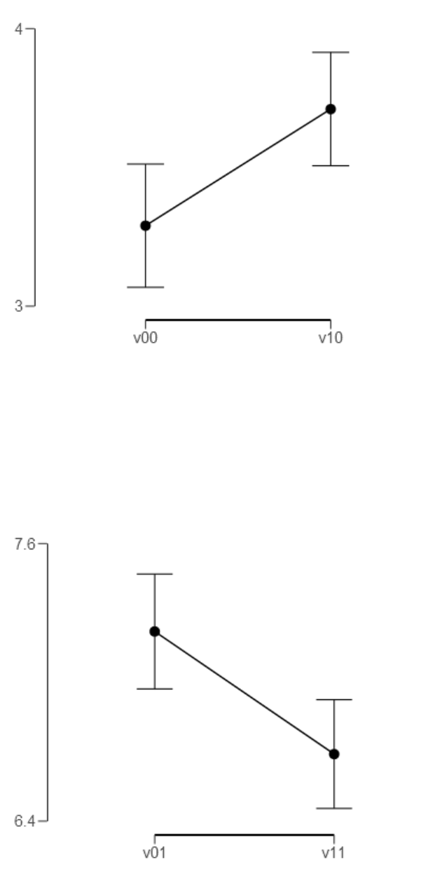
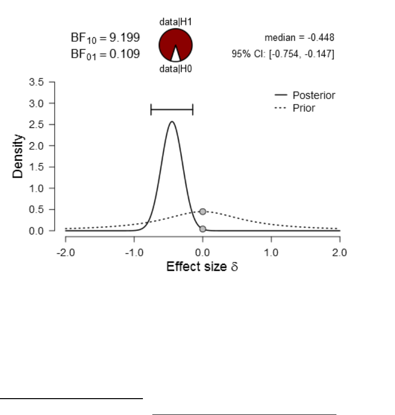
158
Figure 23 provide a visual synopsis of the most essential results of the Bayesian
analysis in a concise format: 1) a visualisation of the prior distribution of the effect
sizes, 2) the associated posterior distributions, 3) the associated 95% Bayesian credible
intervals, 4) the posterior medians, 5) the Bayes Factors, 6) the associated Savage–
Dickey density ratios
120
(E. J. Wagenmakers, Lodewyckx, Kuriyal, & Grasman, 2010),
7) proportion wheels
121
of the Bayes Factor in favour of H
1
.
Figure 22. Prior and posterior plot for the difference between V
00
vs. V
10
.
120
For an interactive visualisation see http://irrational-decisions.com/?page_id=2328
121
The proportion wheels provided an intuitive representation of the strength of evidence associated with
the Bayes factor. The odds are transformed to a magnitude between 0 and 1 and visualised as the
corresponding proportion of the circle. The following analogy has been articulated to facilitate an
intuitive understanding of the “proportion wheel” concept (it has been convincingly argued that analogy
is the core of cognition (Hofstadter, 1982, 1995)): “Imagine the wheel is a dartboard; you put on a
blindfold, the wheel is attached to the wall in random orientation, and you throw darts until you hit the
board. You then remove the blindfold and find that the dart has hit the smaller area. How surprised are
you? The level of imagined surprise provides an intuition for the strength of a Bayes factor.” (E.-J.
Wagenmakers et al., 2017, p. 6)
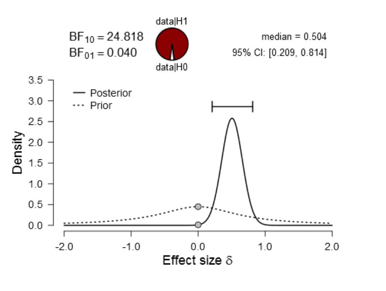
159
Figure 23. Prior and posterior plot for the difference between V
01
vs. V
11
.
In addition, we conducted a Bayes Factor robustness for various Cauchy priors per
pairwise comparison, respectively. Specifically, we contrasted Cauchy priors ranging
from [0, 1.5]. The results are visually summarised in
Figure 24 and
Figure 25, respectively. For the first comparison (V
00
vs. V
10
) the maximum Bayes
Factor was obtained at r ≈ 0.28 (max BF
10
≈ 12.56). For the second comparison (V
01
vs.
V
11
) the maximum evidence in favour of H
1
was associated with r ≈ 0.32 (max BF
10
≈
31.31). Based on this analysis, it can be concluded that the Bayes Factor is robust under
various reparameterizations of r.
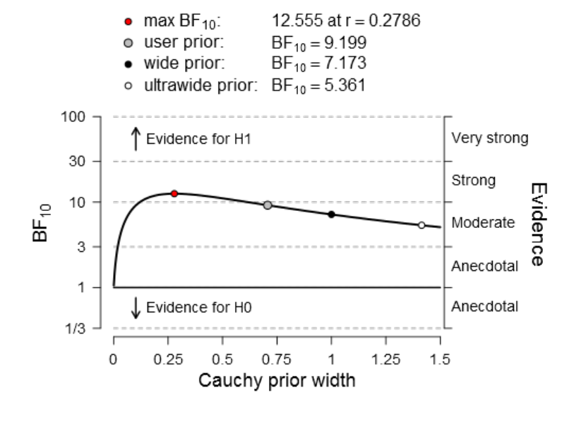
160
Bayes Factor Robustness Check
Figure 24. Visual summary of the Bayes Factor robustness check for condition V
00
vs.
V
10
using various Cauchy priors.
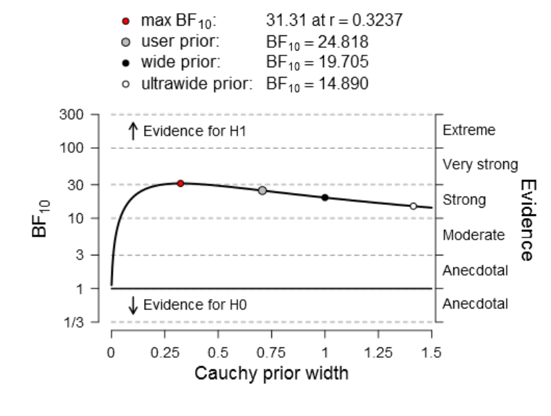
161
Figure 25. Visual summary of the Bayes Factor robustness check for condition V
01
vs.
V
11
using various Cauchy priors.
Furthermore, we carried out a sequential Bayes Factor analysis. This allowed us to
inspect the accumulation of evidence in favour of H
1
as a function of the number of data
points/participants. Prima vista, it can be seen that the evidence in favour of H
1
increases as n accumulates. The results per experimental condition are visualised in
Figure 26 and Figure 27, respectively.
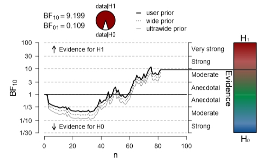
162
Figure 26. Sequential analysis depicting the flow of evidence as n accumulates over
time (experimental condition V
00
vs. V
10
).
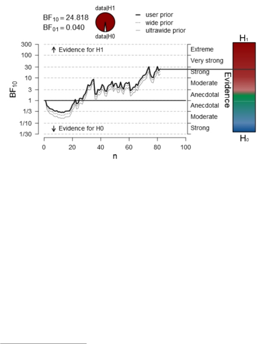
163
Figure 27. The visualisations thus show the evolution of the Bayes Factor (y-axis) as a
function of n (x-axis). In addition, the graphic depicts the accrual of evidence for
various Cauchy priors (experimental condition V
01
vs. V
11
).
A crucial advantage of Bayes Factor analysis over frequentists hypothesis testing is that
in contrast to frequentist NHST (which can only reject H
0
), Bayes Factor analysis
allows to quantify evidence in favour of H
0
(thereby circumventing the inferential
asymmetry associated with NHST). In addition to the graphical and numerical
representation of the evolution of the Bayes Factor (evidential flow) for various prior
choices, we colour-coded
122
the graded BF
10
in favour of H
1
vs. H
0
.
122
The color-coding of the Bayes Factor was accomplished by creating a vector graphic with a gradient
based on a complementary colour triplet (hexadecimal colours: #8B0000, #008B46, #00468B). This
visual representation provides an intuitive “feeling” for the strength of evidence in favour of H
1
and
reduces the demand for abstract though associated with numerical statistical inferences as it maps
numerical values on an intuitively interpretable colour gradient. It has been shown in various contexts that
the format in which statistical information is presented influences subsequent inferential conclusions
(Tooby & Cosmides, 2005; Wason, 1968). From an evolutionary psychology point of view, it has been
argued that logically sound scientific reasoning can be facilitated when information is presented in non-
abstract terms (Baumeister et al., 1998). Statistical inference involves decision-making. Repeated

164
Next, we performed a Bayesian parameter estimation analysis using MCMC methods in
order to obtain precise posterior intervals for all parameters of interest. It should be
noted that the results of both Bayesian approaches do not necessarily converge, that is,
they can lead to diverging inferential conclusions. For instance, when the posterior high
density interval does not include zero the Bayes Factor can contrariwise indicate that H
1
should not be preferred over H
0
. This seemingly paradoxical situation can lead to
confusions and it should be emphasised that Bayesian analysts do not necessarily agree
on which approach to take. While some advocate Bayes Factor analysis, other advocate
the Bayesian parameter estimation approach.
decision-making depletes executive functions (Hagger et al., 2010), that is, the higher-order cognitive
processes which underpin logical thinking are a limited resource (Bechara, Tranel, & Damasio, 2000;
Gailliot, 2008) which can be easily depleted, presumably due to reduction of prefrontal glycogen storage
(de Neys et al., 2013; Kahneman, 2003) – an argument which makes sense in an evolutionary perspective,
i.e., for our ancestors glucose was a limited nutritional resource and we still run this outdated program –
hence we crave it, store it (e.g., obesity), and conserve it whenever possible. In the context of cognitive
depletion and decision-making, it has been empirically demonstrated that the quality of juridical decision-
making is subject to ego-depletion (Danziger, Levav, & Avnaim-Pesso, 2011). Given that hypothesis
testing is in many ways analogous to juridical decision-making, this empirical finding may be transferable
to inferential statistical decision-making. It has been shown in various domains of thinking and reasoning
that humans are “cognitive misers” (Kahneman & Tversky, 1974) and that the quality of decisions is
compromised if this limited (System 2) capacity is overworked (de Neys et al., 2013). Abstract numerical
statistical reasoning is particularly demanding on prefrontal executive functions. Therefore, statistical
information should be presented in an intuitively/heuristically interpretable format whenever this is
possible in order to improve the quality of inferential reasoning. Graphical representation like color-coded
evidence are an effective way to achieve this desideratum. Insights from cognitive linguistics, e.g.,
conceptual metaphor theory (Lakoff, 1993; Lakoff & Johnson, 1980; Lakoff & Nuñez, 2000) can be
successfully utilised to present statistical information in a more intuitive and less error-prone format.
165
2.3.13 Bayesian a posteriori parameter estimation via
Markov Chain Monte Carlo simulations
This section reports the application of Bayesian a posteriori parameter estimation via
Markov Chain Monte Carlo (MCMC) simulations. It has been demonstrated that this
method is a very powerful approach to statistical analysis and inference (Gelman,
Carlin, Stern, & Rubin, 2004). The Bayesian parameter estimation approach can be
regarded as a superior mathematical alternative to conventional NHST t-tests (and
related frequentist methods, e.g., ANOVA). It produces posterior estimates for means,
standard deviations (and their differences) and effect sizes (Kruschke, 2013). In contrast
to the dichotomous decisions which are inferred from conventional t-tests, the Bayesian
parameter estimation approach provides probability distributions of the parameter
values of interest. Furthermore, the Bayesian approach does not rely on the
distributional assumptions which are stipulated by parametric t-tests and it is relatively
insensitive to outliers. In addition, the procedure can be used to calculate credible
intervals around point estimates. For these reasons, it is clearly superior to conventional
NHST (Kruschke, 2013; Kruschke & Liddell, 2015, 2017a; Kruschke & Vanpaemel,
2015).
Specifically, we conducted Bayesian analyses with computations performed by the
Gibbs-sampler JAGS (Plummer, 2005). JAGS is a “flexible software for MCMC
implementation” (Depaoli, Clifton, & Cobb, 2016). We were particularly interested in
measures of central tendency derived from the posterior distribution in order to evaluate
differences between experimental conditions. In addition, we also estimated additional
metrics (e.g., quantiles) of the posterior to gain a more complete picture.
Relatively recent advances in technology make these computationally demanding
methods feasible. The combination of powerful microprocessor and sophisticated

166
computational algorithms allows researchers to perform extremely powerful Bayesian
statistical analyses that would have been very expensive only 15 years ago and virtually
impossible circa 25 years ago. The statistical “Bayesian revolution” is relevant for many
scientific disciplines (Beaumont & Rannala, 2004; S. P. Brooks, 2003; Gregory, 2001;
Shultz, 2007) and the scientific method in general. This Kuhnian-paradigm shift (T.
Kuhn, 1970) goes hand in hand with Moore's law (G. E. Moore, 1965) and the
exponential progress of information technologies (Kurzweil, 2005) (cf. Goertzel, 2007)
and the associated ephemeralization
123
(Heylighen, 2008).
Model comparison via Bayes Factor (Bayesian confirmation theory) as described in the
antecedent section is thus not the only viable Bayesian alternative to classical
frequentist NHST. Bayesian parameter estimation and Bayes Factor analysis differ in
significant ways: Compared to Bayes Factor analysis, the Bayesian parameter
estimation approach provides much richer information because it results in a posterior
probability distribution on all parameters (Bayes Factor analysis does not). Model
comparison and Bayesian parameter estimation are both committed to Bayes’ theorem
as the axiomatic foundation for probabilistic inductive inferences. However, the
questions they address are fundamentally different (Steel, 2007). Whereas model
comparison is concerned with the evaluation (i.e., confirmation/rejection) of
hypotheses, Bayesian parameter estimation is primarily concerned with the computation
of posterior probability distributions for the parameters of interest. However, the
Bayesian parameter estimation approach can also be utilised to test specific research
hypotheses. In the model comparison approach, the decision (accept vs. reject) is based
on a predefined arbitrary threshold (i.e., the strength of the Bayes Factor). In the
123
A concept popularised by Buckminster Fuller which is frequently cited as an argument against
Malthusianism.

167
parameter estimation approach, on the other hand, the inferential decision is based on
the specification of a threshold for the parameter under investigation (viz. a “posterior
high density interval” in combination with a “region of practical equivalence”). The
parameter estimation approach and its associated methods for hypothesis testing will be
described in more detail in the following subsections.
In sum, both Bayesian methods base their decision rules on the posterior distribution.
However, given that they focus on different facets of the posterior distribution the
resulting logical inferences do not necessarily have to coincide (Kruschke, 2014).
Furthermore, both inferential approaches are based on the notion of credence (a
subjective “Bayesian” probability describing the level of confidence or belief). Given
that subjectivity involves the epistemological idiosyncrasies and propensities of a
human cogniser, credence must be regarded as a psychological property.
While hypothesis testing plays a pivotal role in psychology and the biomedical sciences,
it is ancillary in many other scientific disciplines (e.g., physics). Many disciplines that
do not primarily rely on hypothesis testing focus on estimation and modelling. A
common problem in statistical modelling is to estimate the values of parameter of a
given probability distribution. Bayesian Parameter Estimation (BPE) methods provide a
set of powerful and robust statistical tools to obtain these values. In other words, BPE
can produce accurate approximations to the Bayesian posterior distributions of various
parameters (θ, i.e., theta) of interest. That is, parameters are modelled as probability
distributions. BPE utilises computationally expensive Markov chain Monte Carlo
(MCMC) algorithms to achieve this goal. In contrast to NHST, BPE fixes the empirical
data and instead assumes a range of credible values for θ. Moreover, BPE allows
probabilities to represent credibility (i.e., subjective certainty/belief). Hence, a
168
semantically more appropriate alternative nomenclature for BPE (and all other Bayesian
methods) would be “statistical uncertainty modelling”.
In the experimental context at hand, we applied Bayesian parameter estimation methods
to our empirical data in order to obtain accurate estimates of the parameter values of
interest. Based on the a priori defined hypotheses, we were particularly interested in the
posterior distribution of the means per condition, their standard deviations, and the
difference between means. BPE provides informative posterior probability distributions
for all parameters of interest.
In the subsequent subsection we will provide a brief introduction to Bayesian parameter
estimation via Markov chain Monte Carlo methods. After that, we will describe the
actual Bayesian analysis and the results. The section is subdivided as follows (according
to the sequential steps of the analysis):
1. Overview of the utilised software
2. Definition of the descriptive model and specification of priors
3. MCMC computations of the posterior distributions
4. Diagnostics/assessment of MCMC convergence
5. Summary and interpretation of the resulting posterior distributions within the
pertinent theoretical framework
The Bayesian inferential approach we employed provides rich information about the
estimated distribution of several parameters of interest, i.e., it provides the distribution
of the estimates of μ and σ of both experimental conditions and the associated effect
sizes. Specifically, the method provides the “relative credibility” of all possible
differences between means, standard deviations (Kruschke, 2013). Inferential
conclusions about null hypotheses can be drawn based on these credibility values. In

169
contrast to conventional NHST, uninformative (and frequently misleading
124
) p values
are redundant in the Bayesian framework. Moreover, the Bayesian parameter estimation
approach enables the researcher to accept null hypotheses. NHST, on the other, only
allows the researcher to reject such null hypotheses.
The critical reader might object why one would use complex Bayesian computations for
the relatively simple within-group design at hand. One might argue that a more
parsimonious analytic approach is preferable. Exactly this question has been articulated
before in a paper entitled “Bayesian computation: a statistical revolution” which was
published in the Philosophical Transactions of the Royal Society: “Thus, if your primary
question of interest can be simply expressed in a form amenable to a t test, say, there
really is no need to try and apply the full Bayesian machinery to so simple a problem”
(S. P. Brooks, 2003, p. 2694).
The answer is straightforward: “Decisions based on Bayesian parameter estimation are
better founded than those based on NHST, whether the decisions derived by the two
methods agree or not. The conclusion is bold but simple: Bayesian parameter
estimation supersedes the NHST t test” (Kruschke, 2013, p. 573).
Bayesian parameter estimation is more informative than NHST
125
(independent of the
complexity of the research question under investigation). Moreover, the conclusions
drawn from Bayesian parameter estimates do not necessarily converge with those based
on NHST. This has been empirically demonstrated beyond doubt by several
independent researchers (Kruschke, 2013; Rouder et al., 2009).
124
For more detailed information on the frequent logically fallacious misinterpretations of p-values and
related frequentist statistics see chapter xxx.
125
It is also more informative than Bayes factor analysis.

170
2.3.13.1 Software for Bayesian parameter estimation via MCMC
methods
In order to conduct the Bayesian parameter estimation, we utilised several open-source
software packages (all are all freely available on the internet). We created a website
were the associated URLs are compiled: http://irrational-decisions.com/?page_id=1993
Analyses were entirely conducted in R using the “BEST” package (Kruschke, 2014).
Best is an acronym for “Bayesian Estimation Supersedes the t-Test”. Moreover, we
installed JAGS “Just Another Gibbs Sampler” (Plummer, 2003, 2005) and RStudio
(RStudio Team, 2016). BEST has numerous (recursive) reverse dependencies and
reverse import dependencies which can be found with the R code provided in Appendix
E6. The utilised programs have been described in great detail two recent textbooks on
Bayesian analysis (Kruschke, 2010a, 2014).
2.3.13.2 Mathematical foundations of Bayesian inference
Bayesian inference allocates credibility (i.e., belief) across the parameter space Θ
126
of
the model (conditional on the a priori obtained empirical data). The mathematical
axiomatic basis is provided by Bayes’ theorem. Bayes’ theorem derives the probability
of θ given the empirical data in terms of its inverse probability (i.e., the probability of
the data given θ and the prior probabilities of θ). In other word “Bayesian data analysis
involves describing data by meaningful mathematical models, and allocating credibility
to parameter values that are consistent with the data and with prior knowledge”
(Kruschke & Vanpaemel, 2015, p. 279)
126
Uppercase Theta (Θ) denotes the set of all possible combinations of parameter values in a specific
mathematical model (the joint parameter space). Lowercase theta (θ) on the other hand, denotes a single
k-dimensional parameter vector.

171
The mathematical formula for the allocation of credibility across parameters is
axiomatized in Bayes’ theorem (Bayes & Price, 1763), i.e., Bayes’ theorem
mathematically defines the posterior distribution on the parameter values in a formal
manner.
(|) =
(|) ()
()
Where:
• () signifies the prior (the preliminary belief about A)
• () signifies the evidence
• (|) signifies the posterior probability (the belief about of A given B)
• (|) signifies the likelihood.
Applied to the current analysis Bayes’ theorem takes the following form:
(
,
,
,
,
|
)
= ( |
,
,
,
, )
x (
,
,
,
, )
/ ()
Equation 8. Bayes’ theorem (Bayes & Price, 1763) as specified for the hierarchical
descriptive model utilised to estimate θ.
let D be the empirical data, μ
1
and μ
2
the means per experimental condition (e.g.,
condition V
00
and V
10
), σ
1
and σ
2
the associated standard deviations, and the
normality parameter.
Bayes’ theorem emphasises the posterior (conditional) distribution of parameter values
(the Latin terminus “a posteriori” signifies empirical knowledge which proceeds from
experiences/observations). The factors of Bayes’ theorem have specific meaning
172
assigned to them: The “evidence” for the specified model, p(D), equals the total
probability of the data under the model which can be computed by averaging over the
parameter space Θ (Kruschke, 2015). Each parameter value is weighted by the “strength
of belief” in the respective values of θ. For the current model, Bayes’ theorem can be
semantically summarised as follows: It signifies that the posterior probability of the
combination of parameter values (i.e., < μ
1
, μ
2
, σ
1
, σ
2
, >) is equal to the likelihood of
that parameter value combination multiplied by the prior probability of that parameter
combination, divided by the constant p(D). This constant is often referred to as the
“evidence” for the model and is also called the “marginal likelihood function”
(Kruschke, 2013). Its numerical value is calculated by taking the average of the
likelihood, p(D|θ), across all values of θ (i.e., over the entire parameter space Θ),
weighted by the prior probability of θ (Kruschke, 2014). The posterior distribution is
thus always a compromise between the prior believability of the parameter values and
the likelihood of the parameter values, given data. (Kruschke, 2010b). Our experimental
data was measured on a visual analogue scale (VAS) ranging across a continuum of
values. Given the extremely fine-grained nature of our measurements the resulting
numerical values are “quasi-continuous”. Therefore, all parameters are regarded as
continuous variables for all practical purposes. It thus follows that the posterior
distribution is continuously distributed across the joint parameter space Θ (Kruschke et
al., 2017).
Given that Bayesian parameter estimation (BPE) is currently no methodological
standard in psychology we will provide some terminological clarifications of the
underlying Bayesian nomenclature. The credibility of the parameter values after the
empirical observation is termed the “posterior distribution”, and the believability of the
parameter values before the empirical observation is termed the “prior distribution”. The

173
probability of the observation for a particular parameter value combination, is called the
“marginal likelihood function”. It indicates the degree to which the observed outcome is
anticipated, when averaged across all possible values of the weights, scaled
proportionally to their respective believability (Kruschke, 2008). The denominator
labelled as “evidence”, p(D), is the marginal likelihood also referred to as “model
evidence”. In BPE, Bayes’ theorem is used to make inferences about distribution
parameters, i.e., the conditional distribution of θ is calculated given the observed data.
The question is: What is the probability of θ conditional on the observed data? The prior
is an unconditional distribution associated with θ. In contrast to NHST, θ is not assumed
to be random, we are merely nescient
127
of its value. In other words, probability is
conceptualised as a state of subjective belief or state of knowledge (as opposed to
objective “pure” probability as an intrinsic property of θ).
The posterior distribution is approximated by a powerful class of algorithms known as
Markov chain Monte Carlo (MCMC) methods (named in analogy to the randomness of
events observed at games in casinos). MCMC generates a large representative sample
from the data which, in principle, allows to approximate the posterior distribution to an
arbitrarily high degree of accuracy (as ). The MCMC sample (or chain) contains a
large number (i.e., > 1000) of combinations of the parameter values of interest. Our
model of perceptual judgments contains the following parameters: < μ
1
, μ
2
, σ
1
, σ
2
, >
(in all reported experiments). In other words, the MCMC algorithm randomly samples a
very large n of combinations of θ from the posterior distribution. This representative
sample of θ values is subsequently utilised in order to estimate various characteristics of
the posterior (Gustafsson, Montelius, Starck, & Ljungberg, 2017), e.g., its mean, mode,
127
The term “nescienct” is a composite lexeme composed of the Latin prefix from ne "not" + scire "to
know" (cf. “science”). It is not synonymous with ignorant because ignorance has a different semantic
meaning (“to ignore” is very different from “not knowing”).
174
median/medoid, standard deviation, etc. The thus obtained sample of parameter values
can then be plotted in the form of a histogram in order to visualise the distributional
properties and a prespecified high density interval (i.e., 95%) is then superimposed on
the histogram in order to visualise the range of credible values for the parameter under
investigation.
For the current Bayesian analysis, the parameter space Θ is a five-dimensional space
that embeds the joint distribution of all possible combinations of parameter values
(Kruschke, 2014). Hence exact parameter values can be approximated by sampling
large numbers of values from the posterior distribution. The larger the number of
random samples the more accurate the estimate. A longer MCMC chain (a larger
sample) provides a more accurate representation (i.e., better estimate or higher
resolution) of the posterior distribution of the parameter values (given the empirical
data). For instance, if the number of MCMC samples is relatively small and the analysis
would be repeated the values would be significantly different and, on visual inspection,
the associated histogram would appear “edgy”. With larger MCMC samples, the
estimated values (on average) approximate the true values of the posterior distribution
of the parameter values and the associated histogram becomes smoother (Kruschke,
2014). The larger the MCMC sample size the higher the accuracy because the sample
size n is proportional to the “Monte Carlo Error” (MCE; i.e., accuracy is a function of
MCMC sample size). To sum up, the MCMC approach clearly yields approximate
parameter values and its accuracy depends on the number of values n that are used to
calculate the average. Quantitative methods have been developed to measure the Monte
Carlo Error “objectively” (Elizabeth Koehler, Elizabeth Brown, 2009), however, this
intricate topic goes beyond the scope of this chapter. Of great relevance for our purpose
is the fact that this analytic approach also allows to compute the credible difference of

175
means between experimental conditions by computing μ
1
- μ
2
for every combination of
sampled values. Moreover, BPE provides a distribution of credible effect sizes. The
same distributional information can be obtained for the differences between σ
1
and σ
2
(and the associated distributional range of credible effect sizes). To sum up, BPE is
currently one of the most effective statistical approaches to obtain detailed information
about the various parameters of interest.
2.3.13.3 Model specifications – A hierarchical Bayesian descriptive
model
In order to carry out the Bayesian parameter estimation procedure, we first defined the
prior distribution. The to be estimated parameters relevant for the hypotheses at hand
were: the means μ
1
and μ
2
; the standard deviation σ
1
and σ
2
and the normality parameter
ν. We were particularly interested in the a priori predicted difference between
experimental conditions, i.e., μ
1
– μ
2
. The main purpose of the Bayesian parameter
estimation was thus to estimate these parameters and to quantify the associated
uncertainty (i.e., credibility) of these approximations
128
. We defined a descriptive model
for the Bayesian parameter estimation which is outlined in the following subsection. We
ascribed an appropriate prior distribution to all five parameters (see Figure 28)
according to the specification described in Kruschke (2013, 2015; Kruschke &
128
In this situation, Stein’s paradox (2012) is applicable, given that more than three parameters are
estimated simultaneously (i.e., the dimensionality of the multivariate Gaussian distribution Θ is 3). The
mathematical paradox is well-known in decision theory and estimation theory and it points out the
inadmissibility of the he ordinary decision rule for estimating the mean when multiple -variate Gaussian
random vectors are involved
(i.e., if 3). Ergo, in the estimation scenario at hand, the ordinary estimator
^
is a suboptimal
approximation of θ. A compact mathematical proof (based on partial integration) of this counterintuitive
phenomenon has recently been formulised by Samworth (1987; 1981). However, from a pragmatic point
of view, it is still very reasonable to use the empirical data as an estimate of the parameters of interest,
viz., to use
^
as an estimate of θ, since empirical measurements are distorted by independent Gaussian
noise with μ = 0.
176
Meredith, 2012). The prior distribution specified for each parameter is as follows: The
empirical data () is described by a t-distribution (the wider tails make the t-distribution
more robust compared to the Gaussian distribution, i.e., it is less sensitive to outliers).
The t-distribution has three parameters: the mean (μ), the scale parameter (σ), and the
degrees of freedom (ν). Low values of ν are associated with wider tails (ν can be
regarded as a “shape parameter”). As ν get larger the t-distribution converges to a
Gaussian (see Appendix B21 for a visualisation of various ν parametrisations).
In order to make the prior distribution tolerable for a sceptical audience we chose
noncommittal (diffuse) priors which signify a lack of prior knowledge about the
conceivable values of the parameters of interest. Defining the prior distribution in such
vague (noncommittal) terms indicates that it has a negligible impact on the estimation of
the posterior distribution. In other words, by choosing noninformative priors we ensured
that the data governs the inference. All priors were specified according to the model
detailed in Kruschke (2013). For precise mathematical derivations see Kruschke (2014).
2.3.13.4 Definition of the descriptive model and specification of
priors
The parameters μ1 and μ2 are modelled by a normal distribution. In concordance with
Kruscke (2013) the standard deviation of μ was expressed in very broad terms
(SDpooled x 1000). The mean M of the prior distribution of μ was defined a M
pooled
(the
pooled mean of the empirical data). The prior distribution for σ
1
and σ
2
was also
noninformative, i.e., a wide uniform distribution with hyperparameters ranging from
L=SDpooled /1000 to H 1000xSD
pooled
. In practical terms, the resulting priors are
extremely wide and approximate a uniform distribution raging from -∞ to ∞. Lastly, the
prior distribution for a shifted exponential (λ=29, shifted+1) was defined for the
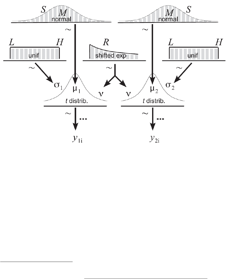
177
normality index ν (for mathematical details see Kruschke, 2013, Appendix A). As a
simplifying assumption, it is postulated that the degree of normality ν is equivalent for
both experimental conditions. The probabilistic model is visualised in Figure 28.
Figure 28. Hierarchically organised pictogram of the descriptive model for the Bayesian
parameter estimation (adaptd from Kruschke, 2013, p. 575)
129
.
Legend:
• S = standard deviation;
• M = mean;
• L =low value;
129
R code for generating pictograms of hierarchical Bayesian models is available on
GitHub under the following URL: https://github.com/rasmusab/distribution_diagrams

178
• H = high value;
• R = rate;
• unif = uniform;
• Shifted exp = shifted exponential;
• distrib. = distribution
The experimental data from condition V
00
(y
1i
) and V
10
(y
2i
) are located at the bottom of
the pictogram. These data are described by heavy tailed and broad (noncommittal) t-
distributions
130
. The data are randomly distributed (~) and the conditions have unique
parameters for the respective means and standard deviations, i.e., μ
1
, μ
2
, and σ
1
, σ
2
,
correspondingly. The parameter for the normality index v is equivalent and thus shared
between conditions. Summa summarum, we defined four unique types of distributions
for the five-dimensional parameter space Θ. The respective distributions were
parametrised in such a way that prior commitment has a minimal impact on the
posterior (i.e., we adopted a non-informative “objective” Bayesian approach).
As can be seen in Figure 29 and Figure 30 the Student t-distribution (invented by
Gosset, 1908; a.k.a. Student)
131
is more centred around 0. In comparison to the Gaussian
distribution, the t-distribution has heavy tails. The height of the tails is denoted by the
Greek letter ν (nu). A heavy-tailed distribution has a large (e.g., a value of 90). A
small on the other hand, signifies an approximation of the Gaussian distribution.
Hence, can be regarded as a quantitative tail-index of a given probability density
function. If has a small parameter, the distribution can represent data with outliers
very well. In the subsequent analysis, data from each experimental condition will be
described with a t distribution. Each condition has its individual mean and standard
130
Note that the t-distribution is stipulated as the distribution for the data. By contrast, the NHST t-test
utilises the t-distribution as a distribution of the sample mean divided by the sample standard deviation.
131
For a historical discussion see Fisher-Box (1938) and Neyman (Meyn & Tweedie, 1993).
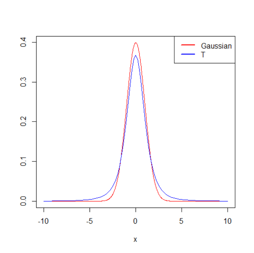
179
deviation. Because we did not observe many extreme values (i.e., spurious outliers) we
will use an identical tail-index ν for both conditions (Kruschke, 2013). In sum, we will
utilise Bayesian estimation for the following five parameters: μ
1
, μ
2
, σ
1
, σ
2
, and .
Figure 29. Visual comparison of the Gaussian versus Student distribution.
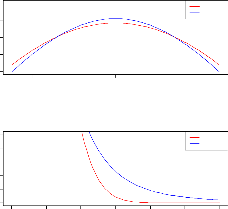
180
Figure 30. Visual comparison of the distributional characteristics of the Gaussian versus
Student distribution.
2.3.13.5 Summary of the model for Bayesian parameter estimation
The specified model describes the data with five parameters: < μ
1
, μ
2
, σ
1
, σ
2
, >. The
priors were very vaguely defined. Noncommittal priors have the advantage that the
parameter estimates are primarily determined by the empirical data (viz., bottom-
up/data driven inference) and not by a priori theoretical considerations which might
-0.4
-0.2 0.0
0.2 0.4
0.90 0.95 1.00 1.05 1.10
x
Gaussian
T
0 1 2 3 4 5 6
0.00 0.02 0.04
x
Gaussian
T

181
bias the model if inaccurate. The analysis willthus produce five parameter estimates that
are statistically plausible given the experimental data at hand.
We parametrised the model with default (noninformative priors) as defined in the
“BEST” R package (Kruschke & Meredith, 2012), specifically we defined normal priors
with a large minimally informative standard deviation for μ, uniform minimally
informative priors for σ, and an minimally informative exponential prior for v.
Mathematical details about this specification are provided in chapter 11 and 12 in
Kruschke (2015).
First, we obtained exact Bayesian estimates for the parameters of interest. We ran the
Metropolis-within-Gibbs sampler with 3 chains, 500 adapt steps (to “tune” the sampler),
1000 burn-in steps
132
and 100000 iterations. We did not use any thinning as this is not a
recommended technique to avoid autocorrelation when sufficient time/computational
resources are available (2013).
2.3.13.6 Markov chain Monte Carlo simulation output analysis and
convergence diagnostics for experimental conditions V
00
and
V
10
As mentioned previously, there are currently no official guidelines for reporting
Bayesian analysis in psychology (Kruschke, 2015). This lack of formal conventions also
holds true for Markov Chain Monte Carlo methods.
133
However, it has been
recommended that convergence diagnostics should be carefully examined and explicitly
132
The general (though questionable) justifications for burning the initial (supposedly invalid) samples is
based on the intention to give the Markov Chain enough time to stabilize to the stationary distribution π
(cf. Meyn & Tweedie, 1993). Using a “random” seed is another alternative to burn-in for choosing an
unbiased starting point.
133
For a remedial attempt concerning the reporting of Monte Carlo methods in structural equation
modelling see Boomsma (2013).
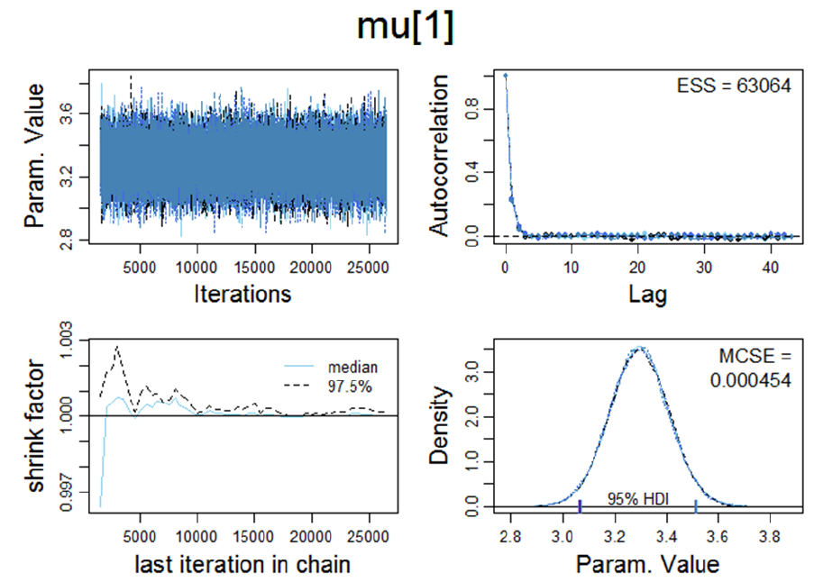
182
reported (Martyn et al., 2016). Given that MCMC sampling forms the basis for the
posterior distribution (which in turn forms the basis for subsequent Bayesian
probabilistic inference) we followed these sensible recommendations and report several
(qualitative and quantitative) diagnostic criteria of convergence. For this purpose, we
utilised the “Coda” package (2004) in R which provides essential functions for
monitoring, summarizing, and plotting the output from iterative MCMC simulations. A
visual summary for experimental condition V
00
is provided in Figure 31 and various
convergence diagnostics will be briefly discussed in the subsequent paragraphs.
Figure 31. Visualisation of various MCMC convergence diagnostics for μ
1
(corresponding to experimental condition V
00
).
Trace plot: In order to examine the representativeness of the MCMC samples, we first
visually examined the trajectory of the chains. The trace plot (upper left panel of Figure
183
31) indicates convergence on θ, i.e., the trace plot appears to be stationary because its
mean and variance are not changing as a function of time. Moreover, the mixing time of
the Markov chain looks satisfactory as the Markov chain appears to rapidly approximate
its steady state distribution.
Density plot: The density plot (lower right panel of Figure 31) consists of a smoothed
(averaged) probability density function. Moreover, the plot entails the 95% HDI and it
displays the numerical value of the Monte Carlo Standard Error (MCSE) of 0.000454.
The Monte Carlo Error (MCSE) is the uncertainty which can be attributed to the fact
that the number of simulation draws is always finite. In other words, it provides a
quantitative index that represents the quality of parameter estimates. For more
information on the Markov chain central limit theorem see Jones (James Flegal,
Hughes, Vats, Dai, & Dootika Vats, 2017). The MCSE package in R provides
convenient tools for computing Monte Carlo standard errors and the effective sample
size (Gelman et al., 2004). Notice that relatively small MCSEs indicate high estimation
precision level. The main idea is to terminate the simulation when an estimate is
sufficiently accurate for the scientific purpose of the analysis. The MCSE at hand is
more than adequate for the purpose at hand. Many practitioners utilize quantitative
convergence diagnostics like the MCSE in addition to visual inspections of trace-plots
to evaluate if the chain has been run long enough.
Shrink factor: Another quantitative metric to check convergence is the shrink factor,
a.k.a. Brooks-Gelman-Rubin statistic (Kruschke, 2014) or “potential scale reduction
factor” denoted with
(left lower panel).
= 1 indicates that the chain is fully
converged. As a heuristic “rule-of -thumb”
> 1.1 indicates that the chains may not
have converged adequality and additional tests should be carried out (Kass, Carlin,

184
Gelman, & Neal, 1998). The mathematical basis of
(based on the between chain
variability) can become complex and is not important for the context at hand.
Theoretically, the larger the number of iterations T, the closer
should approximate 1,
i.e., T ,
1. It can be seen in Table 7 that
1. That is, the qualitatively
presupposed convergence is quantitatively corroborated.
The upper right panel of Figure 31 shows the diagnostics for autocorrelation.
Autocorrelation is a quantitative measure of how much independent information is
contained within a Markov chain. If autocorrelation is high the amount of information
conveyed by each sample is reduced. Consequently, the sample is not representative of
the posterior distribution
134
. Autocorrelation within a chain is the correlation of a value
with subsequent values k steps ahead (Gelman et al., 2004). To quantify autocorrelation,
a copy of the chain is superimposed on its original and the correlations are computed.
The number of steps between the original chain and its copy is termed lag. Hence, the
autocorrelation can be calculated for any arbitrary lag value (or a range of lags). As can
be seen in Figure 31 the autocorrelation function drops steeply around
()
< 3
which indicates a low autocorrelation. The effective sample size (EES) of a Markov
chain is a function of the autocorrelation and hence a metric of information. The ESS
was introduced by (Friendly, Monette, & Fox, 2013) is based on the proportion of the
actual sample size to the amount of autocorrelation. The EES can be utilized to
determine whether the number of Monte Carlo samples is sufficient to produce an
accurate posterior distribution. The MCMC at hand is based on a larger sample
134
One way to counteract MCMC autocorrelation is “thinning” of the Markov Chain. However, this is not
a recommended technique because valuable information is lost which could negatively impact the
accuracy of the estimation of the posterior distribution. A preferable strategy is to produce longer Markov
chains instead.

185
(120000) than the estimated EES of 63064 and we are thus content with this numerical
indicator.
We examined the convergence diagnostics for all other parameters (see Appendix B24
for details), all of which suggested that the desired equilibrium distribution π had been
reached as can be seen in Table 7. Note that 'Rhat' is the potential scale reduction factor
(at convergence, Rhat=1) and 'n.eff' is a crude measure of effective sample size.
Table 7
Summary of selected convergence diagnostics for μ
1
, μ
2
, σ
1
, σ
2
, and ν.
Rhat n.eff
mu1 1 61124
mu2 1 63411
nu 1 22851
sigma1 1 50537
sigma2 1 46096
Note. Because we conducted the analysis multiple times results might vary slightly due
to randomness in the Markov chains.
In sum, the results of our MCMC diagnostic analysis were satisfactory and support the
notion that the stationary distribution is the correct one for a posteriori sampling
purposes. It should be emphasised that no method can conclusively prove convergence
(Plummer, 2003, 2005), that is, it can only be falsified in the Popperian sense. None of
the test batteries discussed above can conclusively “prove” that the MCMC approach
has provided reliable estimates of posterior characteristics. However, we utilised a
diverse battery of MCMC convergence tests and the convergence diagnostics uniformly
suggest convergence to the equilibrium distribution of the Markov chain for all model
parameters (additional diagnostics are reported in Appendix B25 and Appendix B26).

186
Therefore, we proceed with the analysis of the posterior distribution which is described
in the next subsection.
2.3.13.7 Bayesian MCMC parameter estimation for condition V
00
and V
10
Next, we inspected the results of the Bayesian MCMC parameter estimation for
condition V
00
and V
10
. The correlation matrix for all parameters of interest is given in
Figure 32 and the posterior distributions of μ
1
and μ
2
with associated 95% posterior high
density credible intervals is are depicted in Figure 33. The posterior distributions of σ
1
and σ
2
and the Gaussianity parameter ν with associated 95% posterior high density
credible intervals is visualised in Figure 35. The ROPE and HDI-based decision
algorithm is explained in Appendix B22.
Table 8
Results of Bayesian MCMC parameter estimation for experimental conditions V
00
and
V
10
with associated 95% posterior high density credible intervals.
mean median mode HDI% HDIlo HDIup compVal %>compVa
l
mu1 3.2939 3.2940 3.2869 95 3.073 3.524
mu2 3.7102 3.7103 3.7215 95 3.507 3.917
muDiff -0.4163 -0.4170 -0.4320 95 -0.722 -0.111 0 0.36
9
sigma1 0.9970 0.9923 0.9835 95 0.836 1.173
sigma2 0.9132 0.9091 0.9054 95 0.761 1.071
sigmaDiff 0.0838 0.0834 0.0896 95 -0.139 0.309 0 77.19
7
nu 43.2890 34.9173 18.8500 95 5.046 105.167
log10nu 1.5356 1.5430 1.5465 95 0.952 2.105
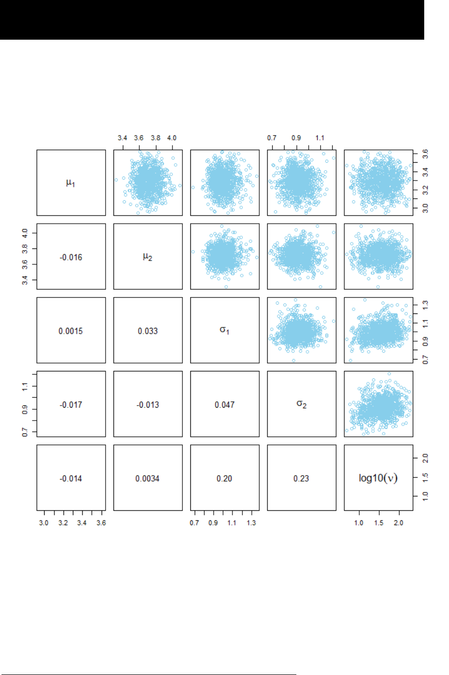
187
effSz -0.4363 -0.4365 -0.4338 95 -0.759 -0.115 0 0.36
9
Figure 32. Correlation matrix for the estimated parameters (μ
1
, μ
2
, σ
1
, σ
1
, ν) for
experimental condition V
00
and V
10
.
A high-resolution vector graphic is available under the following URL as a PDF:
http://irrational-decisions.com/phd-thesis/cor-matrix-exp1.pdf
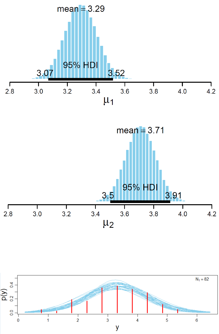
188
Figure 33. Posterior distributions of μ
1
(condition V
00
, upper panel) and μ
2
(condition
V
10
, lower panel) with associated 95% posterior high density credible intervals.
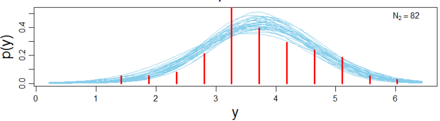
189
Figure 34. Randomly selected posterior predictive plots (n = 30) superimposed on the
histogram of the experimental data (upper panel: condition V
00
; lower panel condition
V
10
).
Figure 36 shows the plot for the “posterior predictive check”. The graphic depicts
curves that were produced by selecting random steps in the MCMC chain and plotting
the t distribution (with the corresponding values of μ, σ and ν for that step). In total n =
30 representative t-distributions are superimposed on the histogram of the actual
empirical dataset. The upper panel of
Figure 36 corresponds to condition V
00
(μ
1
) and the lower panel to the samples for
condition V
10
(μ
2
). This combinatorial graphic thus allows to visually inspect if the
model has a good fit with the experimental data. It can be seen that the specified model
provides an accurate approximation for the centrality parameters of interest, i.e., the
“goodness-of-fit” is heuristically satisfactory as there is little discrepancy between the
estimated values and the empirical data.
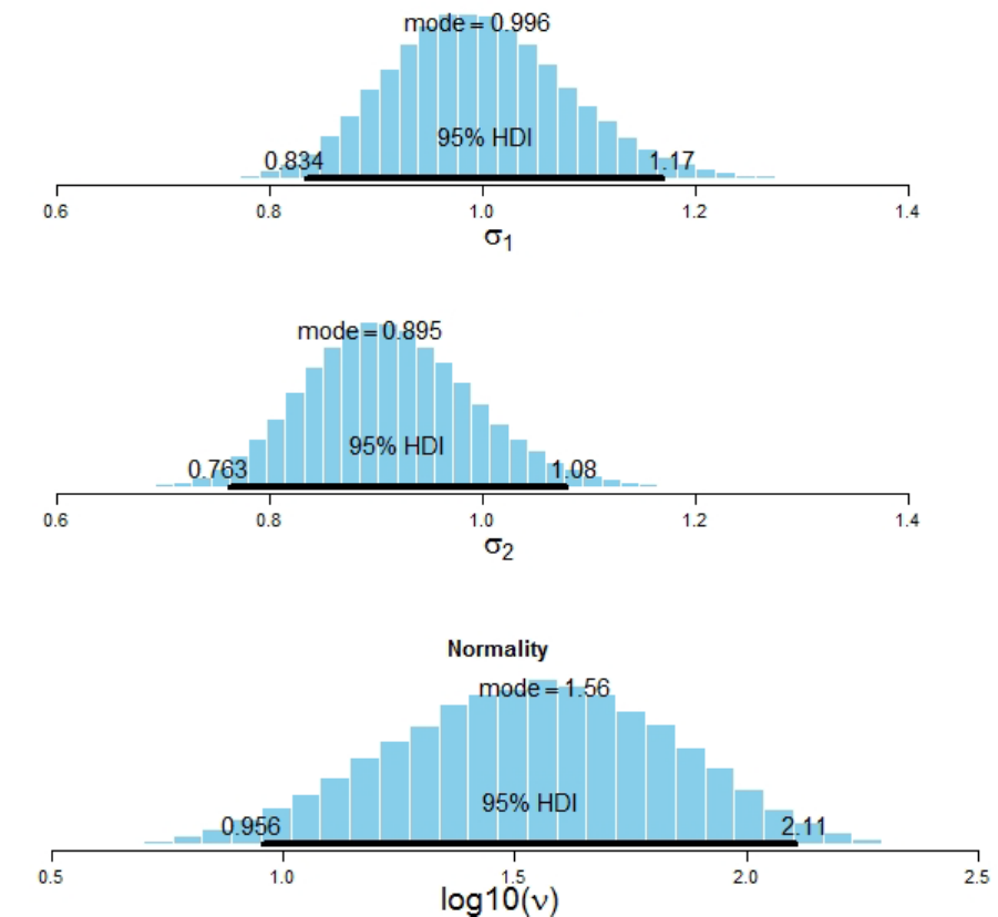
190
Figure 35. Posterior distributions of σ
1
(condition V
00
, upper panel), σ
2
(condition V
10
,
lower panel), and the Gaussianity parameter ν with associated 95% high density
intervals.
2.3.13.8 Bayesian MCMC parameter estimation for the mean
difference between condition V
00
and V
10
After obtaining exact posterior estimates for all parameters, we modelled the mean
difference between condition V
00
and V
01
. For this purpose, we ran another MCMC
simulation with 100000 iterations, 500 adaptation steps, and 1000 burn-in steps. We did
not apply any thinning to the Markov chain and ran multiple chains in parallel (with the

191
exploitation of multi-core CPUs). A visual summary of the posterior distribution of the
estimated difference between means is provided in Figure 36
Figure 36. The posterior predictive plot indicated a good fit (as illustrated in Figure 37).
We prespecified a ROPE centred around zero with a radius of 0.1. As can be seen in
Figure 36, the ROPE did not overlap with the 95% HDI. Thus, we concluded that the
credible difference between mean is unequal to zero and we rejected H
0
based on this
decision algorithm. We also examined the credible range of the effect size associated
effect size and constructed a ROPE ranging from [-0.1, 0.1] arounds its null value.
Again, the ROPE did not overlap with the HDI. In addition, we modelled the standard
deviation of the difference between means which resulted in an estimated value of ≈
1.22 (95% HDI ranging from [1.01, 1.43]). A numerical summary of the results is given
in Table 9. A complete high-resolution synopsis can be accessed under the following
URL: http://irrational-decisions.com/phd-thesis/summary-exp1-cond-v00-vs-v10.pdf
Based on this analysis, we concluded that the credible difference between mean is ≈ -
0.43 with a 95% HDI ranging from [-0.70, -0.15]. The associated effect size was
estimated to be ≈ -0.36 and the associated 95% HDI spanned [-0.56 -0.12]. We utilised
the 95% HDI in combination with a predefined ROPE in order to make a dichotomous
decision concerning our a priori hypothesis. The results cross-validated those obtained
in our previous analyses and provided additional valuable information about the
empirical data at hand which was unavailable in the NHST and Bayes Factor
framework, thereby significantly increasing the precision of our statistical inferences.
Table 9
Numerical summary of the Bayesian parameter estimation for the difference between
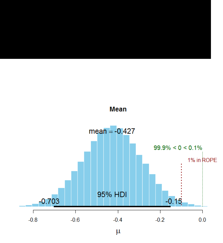
192
means for experimental condition V
00
vs. V
01
with associated 95% posterior high density
credible intervals.
mean median mode HDI% HDIlo HDIup compVal %>compVal
mu -0.427 -0.426 -0.425 95 -0.703 -0.150 0 0.138
sigma 1.218 1.214 1.201 95 1.013 1.435
nu 40.629 32.475 16.432 95 3.368 101.342
log10nu 1.494 1.512 1.553 95 0.835 2.092
effSz -0.353 -0.353 -0.357 95 -0.592 -0.118 0 0.138
Figure 36. Visual summary of the Bayesian parameter estimation for the difference
between means for experimental condition V
00
vs. V
01
with associated 95% HDI and a
ROPE ranging from [-0.1, 0.1].
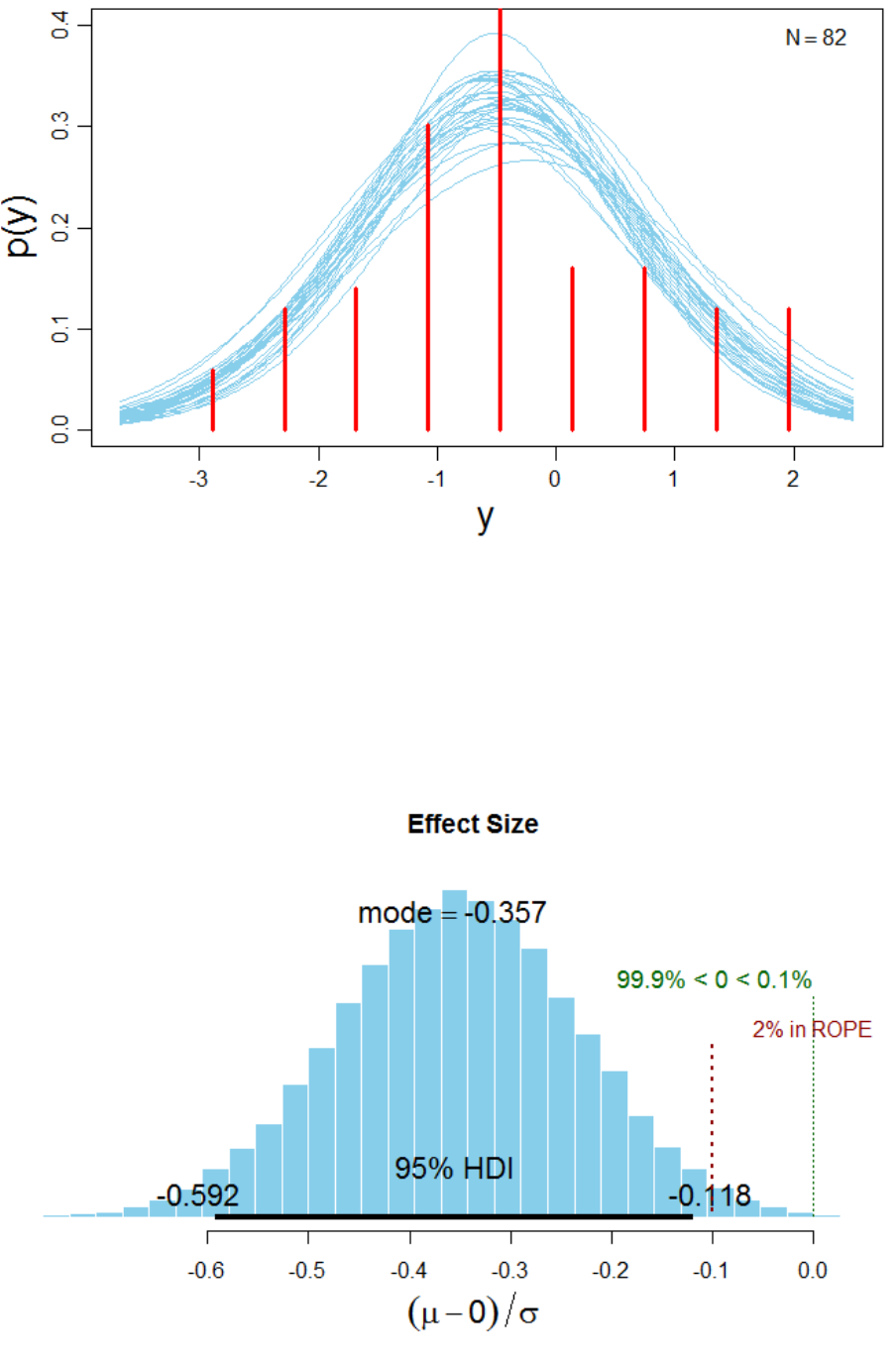
193
Figure 37. Posterior predictive plot (n=30) for the mean difference between
experimental condition V
00
vs. V
01
.
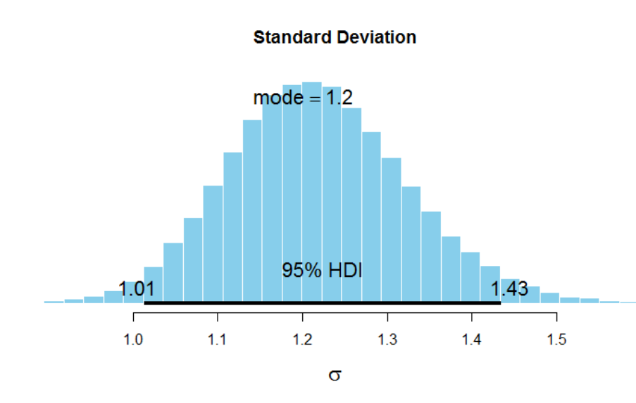
194
Figure 38. Visual summary of the Bayesian parameter estimation for the effect size of
the difference between means for experimental condition V
00
vs. V
01
with associated
95% HDI and a ROPE ranging from [-0.1, 0.1].
Figure 39. Visual summary of the Bayesian parameter estimation for the standard
deviation of the difference between means for experimental condition V
00
vs. V
01
with
associated 95% HDI and a ROPE ranging from [-0.1, 0.1].
2.3.13.9 Markov chain Monte Carlo simulation output analysis and
convergence diagnostics for experimental conditions V
01
and
V
11
Next, we focused on the difference between experimental conditions V
01
and V
11
. For
reasons of brevity, we do not report the individual parameter estimates and focus
immediately on the difference between means in order to evaluate our hypothesis.

195
We thus proceed with our analysis of the difference between means of condition V
01
and V
11
. We ran the MCMC simulation with the same specification as reported before
(burn-in=1000, adaptation=500, iterations=100000). The convergence diagnostics
indicated that the equilibrium distribution π had been reached. The estimated mean
difference between experimental conditions V
01
and V
11
was ≈ 0.54 with an associated
HDI ranging from [0.23, 0.84]. The a priori constructed ROPE [-0.1, 0.1] did not
overlap with the 95% HDI, thereby corroborating our initial hypothesis (i.e., based on
this decision procedure H
0
can be rejected and H
1
is accepted). The associated effect
size was estimated to be ≈ 0.41 (95% HDI ranging from [0.16, 0.65]) and the ROPE
confirmed the (idiosyncratic) practical significance of this value. The results are
summarised in numerical form in Table 10. A visual synopsis is illustrated in Figure 40.
Table 10
Numerical summary of the Bayesian parameter estimation for the difference between
means for experimental condition V
10
vs. V
11
with associated 95% posterior high density
credible intervals.
mean median mode HDI% HDIlo HDIup compVal %>compVal
mu 0.537 0.537 0.532 95 0.227 0.839 0 100
sigma 1.338 1.336 1.347 95 1.073 1.606
nu 32.035 23.196 9.339 95 2.080 89.091
log10nu 1.356 1.365 1.438 95 0.638 2.037
effSz 0.406 0.404 0.406 95 0.164 0.654 0 100
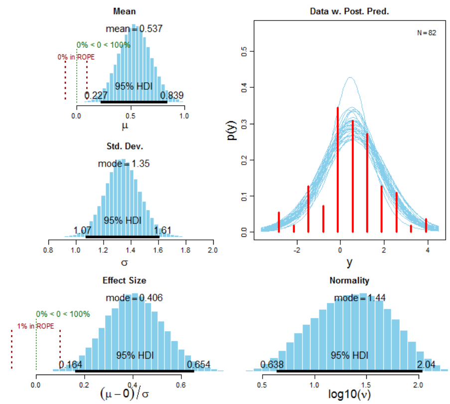
196
Figure 40. Visual summary of the Bayesian parameter estimation for the difference
between means for experimental condition V
10
vs. V
11
with associated 95% HDIs and a
ROPEs ranging from [-0.1, 0.1].
2.4 Discussion
The results of this experiment confirmed our a priori predictions and demonstrate
noncommutativity effects in psychophysical visual judgments. Moreover, they are in
line with the general predictions formulated by Atmanspacher and colleagues
(Atmanspacher, 2014, 2016; Atmanspacher & Römer, 2012b). Prima vista, the
197
observed noncommutativity effects might seem “irrational” but only if the results are
analysed in isolation. However, if the results are conditionalized on the entire contextual
situatedness of the experiment, the results make sense. Any type of measurement, (be it
physical, psychological, or psychophysical) is always embedded in a specific context
and this context significantly influences the measurement in question. It follows that
measurements should never be considered in isolation. This holistic conceptualisation of
scientific measurements is congruent with Nils Bohr’s Copenhagen interpretation of
quantum mechanics (Filliben, 1975). Moreover, the Kolmogorovian notion of sample
space assumes a single sample space for the entire universe. It should be emphasised
that Kolmogorov himself did not defend this notion. In quantum mechanics, sample
spaces are modelled as n-dimensional (compatible/incompatible) Hilbert spaces. This
multidimensionality allows to incorporate results which appear paradoxical (irrational)
in a unidimensional sample space (but see Busemeyer & Bruza, 2012). In sum, our
results support the prediction that “non-commuting operations must be expected to be
the rule rather than the exception for operations on mental systems” (Atmanspacher,
2014a, p. 24). To our best knowledge, the present psychophysics experiment is the first
systematic investigation of noncommutativity in sequential visual perceptual judgments.
The present data can be integrated into a progressively accumulating corpus of scientific
literature which empirically illustrates that quintessential quantum mechanical
principles like superposition, complementarity, and entanglement are applicable beyond
the physical micro domain (Atmanspacher, 2012; Atmanspacher & Filk, 2013;
Atmanspacher & Römer, 2012; beim Graben, 2013; Blutner et al., 2013; Busemeyer et
al., 2011a; Kvam, Pleskac, Yu, & Busemeyer, 2015; Z. Wang et al., 2013). Our findings
particularly highlight the importance of non-commutative structures in the measurement
of psychophysical observables (cf. Atmanspacher, 2016).
198
Specifically, the data indicates that low luminance stimuli were on average rated
significantly lower when anteceded by equivalent stimuli, relative to low luminance
stimuli anteceded by high luminance stimuli (M
Δ
=-0.42). On the other hand, the
brightness of high luminance stimuli was on average rated significantly higher when the
high luminance stimuli were anteceded by low luminance stimuli relative to high
luminance stimuli anteceded by equivalent stimuli (M
Δ
=-0.53). In the current
experimental context, the most relevant difference between classical and quantum
probability models is the way in which they deal with violations of the commutativity
axiom (see Atmanspacher, 2014a). That is, the quantum model allows for violations of
symmetry because observables do not have to commute. In other terms, the defining
difference between classical probability theory and quantum probability theory is
noncommutativity of cognitive operators. If projectors do commute, classical
Kolmogorovian/Boolean probability theory applies, “iff” (if and only if) they do not
commute, quantum probability applies. Consequently, the present results can be
parsimoniously accounted for in the quantum framework whereas classical cognitive
models have to utilise (non-parsimonious) auxiliary hypotheses to explain the results
post festum (see Discussion section 6.2 for a more elaborate version of this argument in
the context of the Duhem-Quine Thesis). Furthermore, the quantum model makes the
prediction (noncommutativity of cognitive operations) a priori (an important aspect of
hypothesis testing which allows for prespecified planned post-hoc comparisions) as
noncommutativity is a defining feature of this explanatory framework. Indeed, is has
been argued that noncommutative operations are ubiquitous in psychology and related
areas (Atmanspacher, 2014a; Atmanspacher & Filk, 2013; Atmanspacher & Römer,
2012; beim Graben, 2013). Our results are thus commensurate with those discussed in
the previous section (i.e., section 1.12) and can be interpreted as a QQ-equality because
199
the psychophysical results display the same ordering schema as the Gallup poll
described before (viz., “Clinton followed by Al Gore” versus “Al Gore followed by
Clinton). As discussed before, classical probability theory cannot easily account for this
kind of order effects because events are represented as sets and are stipulated to be
commutative, that is, P (A ∩ B) = P (B ∩ A). The data of Experiment 1 thus violates the
Kolmogorovian commutativity axiom which is central to the majority of
cognitive/computation models. Quantum models of cognition can thus parsimoniously
account for these prima facie "irrational/paradoxical" judgment and decision-making
phenomena and indeed predicts them a priori. The current experiment thus provides
corroborating empirical evidence for the validity of the predictions derived from the
quantum model.
CHAPTER 3. EXPERIMENT #2:
CONSTRUCTIVE MEASUREMENT EFFECTS
IN SEQUENTIAL VISUAL PERCEPTUAL
JUDGMENTS
3.1 Experimental purpose
Our previous experiment provided empirical support for the QP prediction that
sequential introspective psychophysical judgments are noncommutative (cf.
Atmanspacher, 2014a; Z. Wang et al., 2014). However, the experimental design left
some important questions unresolved. Specifically, one outstanding empirical question
in relation to the previous analysis is the following: Does the mere act of performing a
psychophysical measurement have a constructive effect which influences subsequent
psychophysical measurements? Recent empirical research in the domain of affective
200
(White et al., 2014b) and attitudinal judgments (White et al., 2015) suggests that this is
the case. As discussed before, conceptually related results have also been reported in
various other domains (e.g., Trueblood & Busemeyer, 2011; Z. Wang & Busemeyer,
2013; Z. Wang et al., 2014).
Based on this theoretical and empirical background, we formulated several a priori
hypotheses concerning the constructive role of psychophysical measurements.
Specifically, we were interested to experimentally test whether providing a
psychophysical judgement for a high vs. low luminance visual stimulus exerts a
constructive influence on a subsequent psychophysical judgment of an oppositely
valued visual stimulus.
An additional objective of the present experiment was to conceptually replicate and
cross-validate the previously discussed results reported by White et al. (2014b, 2015) in
a completely different context. Given that affective and attitudinal evaluation are
higher-order cognitive processes, we employed a more controlled experimental
approach in order to establish the robustness of the QP principles at a more fundamental
perceptual level. The main advantage of a low-level psychophysical approach is that
differences in visual stimulus intensity can be varied quantitatively in a much more
controlled and systematic fashion (as compared to the compound stimuli used in the
experiments by White et al., 2014b; 2015). Another methodological/statistical
advantage of the psychophysics approach towards noncommutativity is that it provides
a significantly larger dataset because psychophysical measurements can be recorded in
rapid succession. Moreover, science possesses much more detailed knowledge about the
workings of the perceptual systems, as compared to the much more complex higher-
order cognitive processes which are thought to underpin affective and attitudinal
judgments. Therefore, we approached the question of whether judgments exert
201
constructive effects in psychological measurements from a more reductionist
psychophysical point of view. From a reductionist point of view, research should
progress in an incremental manner – starting at the most fundamental level and
gradually move up to more complex systems. Once an empirical foundation has been
firmly established at a low level one can subsequently move up to the next level in the
cognitive processing hierarchy to explore more complicated compound higher-level
cognitive processes. For this purpose, we designed a psychophysics laboratory task in
order to isolate and empirically investigate the psychophysical mechanism of interest.
3.2 A priori hypotheses
Our hypotheses were formulated a priori and they were derived from the pertinent
quantum cognition literature (Atmanspacher, 2014a, 2016; Atmanspacher & Römer,
2012; Z. Wang et al., 2013; White et al., 2015; White, Pothos, & Busemeyer, 2014a).
The experimental conditions in our design conceptually correspond to the positive vs.
negative affective valence conditions in (White et al., 2014b)
The directional a priori hypotheses of primary interest were:
H
1
: Measuring subjectively perceived brightness of a high luminance stimuli first (i.e.,
binary measurement condition) produces a decrease in subsequent psychophysical
measurement of a low luminance stimuli as compared to the singular measurement
condition.
H
2
: Measuring the subjectively perceived brightness of a low luminance stimuli first
produces an increase in the subsequent psychophysical measurement relative to the
singular measurement condition.
202
In symbolic form the hypotheses can be expressed as follows:
H
:
>
H
:
<
where
V
00
= high luminance stimuli → low luminance stimuli (singular measurement)
V
01
= high luminance stimuli → low luminance stimuli (binary measurement)
V
10
= low luminance stimuli → high luminance stimuli (singular measurement)
V
11
= low luminance stimuli → high luminance stimuli (binary measurement)
Note that our prime objective was not to demonstrate noncommutativity in
psychophysical judgments (this was the main purpose of Experiment 1). Rather, this
experiment was designed to elucidate the potentially constructive influence of an
intermediate psychophysical judgment on a subsequent one. Both hypotheses were
logically derived from the predictions of the QP model (Pothos & Busemeyer, 2013).
3.3 Method
3.3.1 Participants and Design
The experiment was conducted in the psychology laboratory of the University of
Plymouth (United Kingdom) and ethical approval was obtained from the universities
human research ethics committee. Seventy psychology students from the University of
Plymouth participated in this study (45 women and 25 men, ages ranging between 18
and 29 years, M
age
= 21.79; SD
age
= 4.54). Students were recruited via the cloud-based

203
Participant Management Software (Sona Experiment Management System®, Ltd.,
Tallinn, Estonia; http://www.sona-systems.com) which is hosted on the universities
webserver. In addition, a custom-made website was designed in HTML to advertise the
study in an attractive way to the student population (URL: http://irrational-
decisions.com/sona/qp.html). All participants received course credit for their
participation.
3.3.2 Apparatus and materials
The experiment was isomorphic to Experiment 1, except for a single experimental
parameter, i.e., we systematically varied the presence or absence of intermediary
psychophysical measurements in a counterbalanced manner (as described below).
3.3.3 Experimental Design
The basic structure of the experiment was a 2(measurement condition: singular rating
vs. binary measurement) x 2(stimulus order: high luminance → low luminance vs. low
luminance → high luminance) repeated measures factorial design as schematized in
Figure 41. The dependent measure was the condition dependent brightness rating which
was recorded on a visual analogue scale (VAS) (Aitken, 1969) identical to Experiment
1.
3.3.4 Experimental procedure
Before the commencement of the experiment, participants were briefed and accorded
informed consent. Subsequently, participants were seated in front of a personal and
received further instructions.

204
3.3.5 Sequential visual perception paradigm
Similar to Experiment 1, we first collected general demographic information. Then, the
visual perception paradigm was initiated. Before the beginning of the experimental
trials, participants completed a practice block consisting of 4 trials. During the practice
phase, participants were acquainted with the workings of the VAS and the general
experimental procedure. After that, the experimental block was automatically initiated.
A single experimental trial consisted of the successive presentation of two stimuli. A
pair of stimuli always consisted of opposing luminance levels, that is, low luminance
was always followed by high luminance and vice versa. Each stimulus was presented
for 60 frames (≈ 1 seconds)
135
. In 50% of the trials participants were requested to rate
the brightness of the first stimulus (intermediate measurement) and subsequently the
second rectangle (final measurement). In the remaining trials participants were
presented with the first stimulus but were informed that no rating was required (singular
measurement condition). After a manual response was emitted (single left mouse click),
the second stimulus appeared which consistently required a VAS rating response. In
other terms, the task of participants was to evaluate the visual stimuli under different
instructional sets. Hence, for half of the trials participants were required to evaluate the
brightness of both stimuli whereas for the other half they only had to judge the second
stimuli. In the PsychoPy backend, trials were organised into two blocks. The first block
contained the “intermediate (i.e., binary) measurement condition" and the second block
the “no intermediate (i.e., singular) measurement condition". Both blocks were
programmatically enclosed within a loop which enabled randomization of block
135
Vertical refresh rate of screen = 60Hz.
1 frame = 1000ms/60 ≈ 16.67ms (frame to frame variability on average = 2.18ms)
205
presentation order. In addition, trial order within each block was randomized within
participants. Randomization was archived by utilising the Python "NumPy" package
(Van Der Walt et al., 2011) and its relevant randomization functions. The exact
temporal sequence of events within each experimental trial is schematically depicted in
Figure 41.
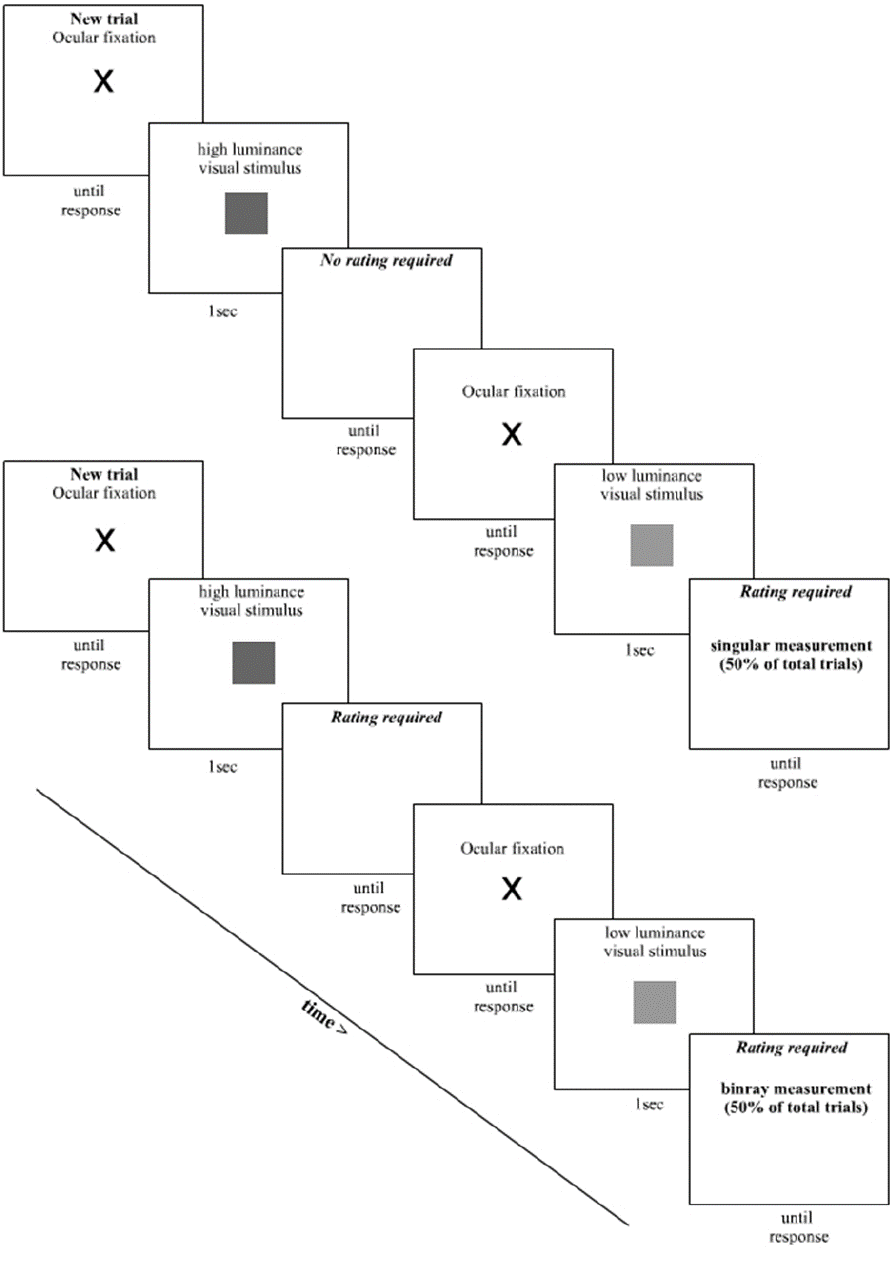
206
Figure 41. Schematic visualisation of the temporal sequence of events within two
successive experimental trials.
207
The within-trial sequence of events was as follows: Initially, a white fixation cross was
displayed on a black background until a manual response was emitted (single left
mouse-click). The following instructions were presented to participants: “New trial:
Please fixate the cross with your eyes and click the mouse when you are ready”. Next, a
rectangle of either high or low luminance appeared in the centre of the screen (screen
size = 1920 x 1080, the application was executed in fullscreen mode) with a fixed
duration of 120 frames. The rectangle was then replaced by either a rating request or no
rating request, (i.e., singular vs. binary measurement condition) which was presented
until a response was emitted (either a rating on the VAS or a mouse-click response,
depending on the respective condition). After that, the second rectangle appeared for the
same temporal duration followed by the final rating request. In sum, participants
completed a total of 300 experimental trials.
Upon completion of the experiment, participants were debriefed and were given the
possibility to ask questions concerning the purpose and theoretical background of the
study. Finally, participants were thanked for their cognitive efforts and released.
3.4 Statistical Analysis
We utilised the same analyses as in the previous experiment, i.e., NHST analysis, Bayes
Factor model comparison, and MCMC-based Bayesian parameter estimation. For
reasons of parsimony and to avoid repetition, we refer to the preceding chapter for
further details. As expounded above, the subsequent analyses exclusively focus on the
postulated constructive role of psychophysical measurements (White et al., 2015,
2014b).

208
3.4.1 Frequentist NHST analysis
We first tested if the Gaussianity assumption which underpins parametric testing
procedures was satisfied. We utilised the R package “moments”
136
to evaluate
skewness
137
and kurtosis
138
of the sample distributions. Both distributional
characteristics were within the normal range of ±2 and ±7, respectively (cf. Cain et al.,
2016; Groeneveld & Meeden, 1984), indicating that the data is neither saliently skewed
nor kurtotic. In addition, Shapiro-Wilk tests indicated that the differences between
means is normally distributed (see Table 11). Visual inspection of the distributional
characteristics of the data using Q-Q plots qualitatively corroborated the quantitative
results (see Appendix B8 for plots and additional indices). We then proceeded to test the
relevant hypotheses with two paired samples t-test (bidirectional). Associated
descriptive statistics are depicted in Table 12.
Table 11
Shapiro-Wilk’s W test of Gaussianity.
W
p
V
00
-
V
01
0.990
0.855
V
10
-
V
11
0.995
0.995
Note. Significant results suggest a deviation from normality.
136
The associated CRAN URL of the R package is as follows: https://cran.r-
project.org/web/packages/moments/
137
The corresponding formula for the Fisher-Pearson coefficient of skewness is as follows (see also Doane
& Seward, 2011).:
(
)
/
, where signifies the mean, s the standard deviation, and N the number of data points
138
The definition of Pearson’s measure of kurtosis is:
(
)
/
, where signifies the mean, s the standard deviation, and N the number of data points.

209
Table 12
Descriptive statistics for experimental conditions.
N
Mean
SD
SE
V
00
70
3.820
1.020
0.122
V
01
70
3.290
1.020
0.122
V
10
70
6.630
1.010
0.121
V
11
70
7.110
1.010
0.121
Variable declarations:
V
00
= high luminance stimuli → low luminance stimuli (singular measurement)
V
01
= high luminance stimuli → low luminance stimuli (binary measurement)
V
10
= low luminance stimuli → high luminance stimuli (singular measurement)
V
11
= low luminance stimuli → high luminance stimuli (binary measurement)
Both t-test were statistically significant. The first comparison indicated that V
00
was
rated significantly higher relative to V
01,
M
Δ
=-0.53; t(69)=-2.96, p=0.004, 95%CI [0.17,
0.89]; Cohen’s d=0.35, 95%CI
for d [0.11, 0.59]. On the other hand, V
10
was rated
significantly lower as compared to V
11
M
Δ
=-0.48; t(69)=-2.96, p=0.005, 95%CI [-0.81, -
0.15]; Cohen’s d=-0.34, 95%CI
for d [-0.58, 0.10]. A comprehensive tabular summary
is provided in Table 13 and the data is visualised in Figure 42 and Figure 43.
139
Taken
139
In addition, a complete summary of the results and an interactive visualisation of the associated Vovk-
Sellke maximum p-ratio (Sellke et al., 2001; Vovk, 1993) is provided under the following URL as a
HTML-file: http://irrational-decisions.com/phd-thesis/exp2/frequentist-analysis-exp2.html
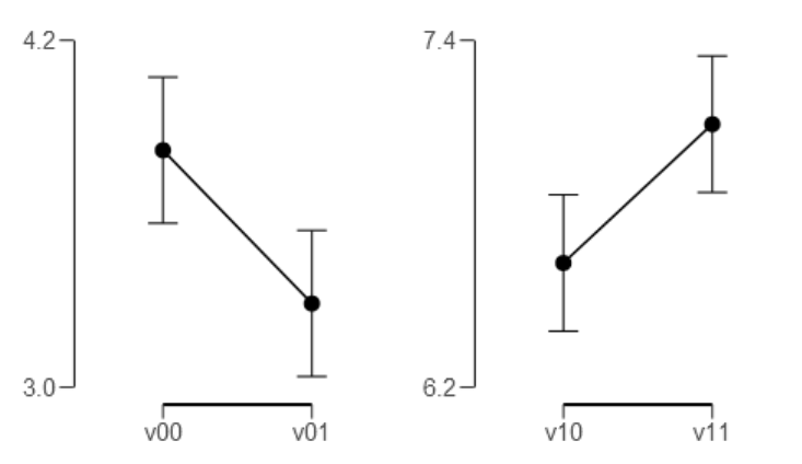
210
together, the results corroborate our a priori hypotheses and provide a conceptual cross-
validation of the findings reported by (White et al., 2015, 2014b).
Figure 42. Visual summary of differences between means with associated 95%
confidence intervals.
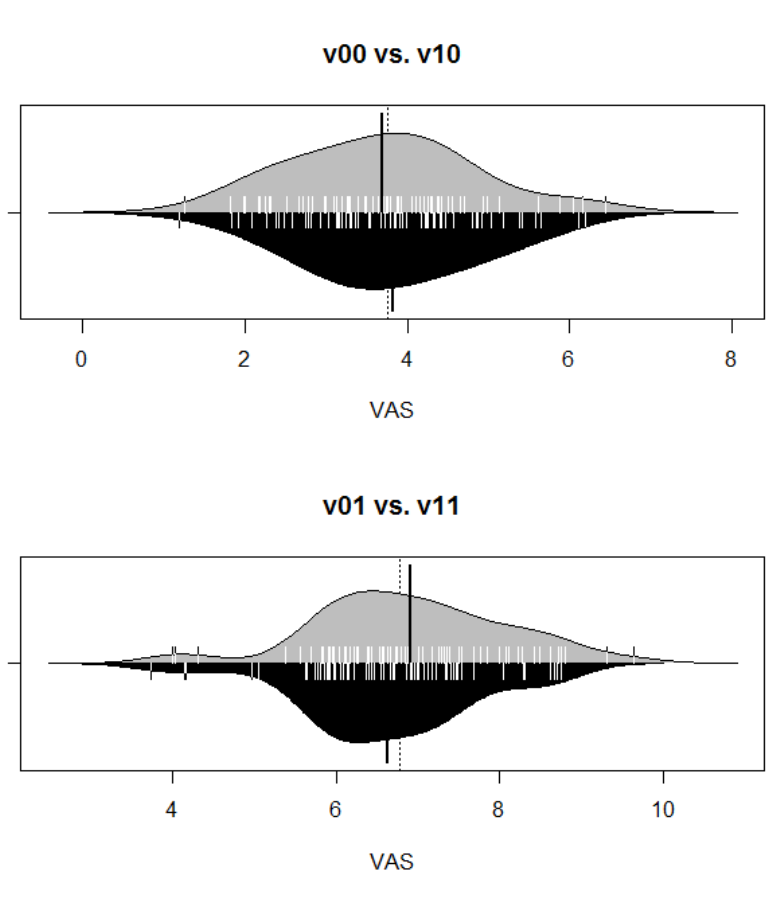
211
Figure 43. Asymmetric beanplots (Kampstra, 2008) depicting the differences in means
and various distributional characteristics of the dataset.
Note: The thin horizontal lines represent individual data points and the thick black line
indicates the grand mean per condition. The shape of the bean visualises the density of
the distributions (Gaussian kernel). It can be seen the beanplots provide much more
detailed information about the data as compared to classical boxplots (but see
Juutilainen et al., 2015).

212
Table 13
Paired samples t-tests and nonparametric Wilcoxon signed-rank tests.
95% CI for Location
Parameter
95% CI for
Effect Size
Test
Statistic
df
p
VS-
MPR*
Location
Parameter
SE
Difference
Lower
Upper
Effect
Size
Lower
Upper
v00
-
v01
Student
2.960
69
0.004
15.944
0.530
0.179
0.173
0.887
0.354
0.111
0.594
Wilcoxon
1687.000
0.009
8.409
0.520
0.126
0.872
0.358
0.104
0.568
v10
-
v11
Student
-2.871
69
0.005
12.977
-0.480
0.167
-0.814
-0.146
-0.343
-0.583
-0.101
Wilcoxon
766.000
0.005
13.162
-0.481
-0.834
-0.151
-0.384
-0.587
-0.134
* Vovk-Sellke Maximum p -Ratio: Based on the p -value, the maximum possible odds in favor of H over H equals 1/(-e p log( p ))
for p ≤ .37 (Sellke, Bayarri, & Berger, 2001).
Note. For the Student t-test, location parameter is given by mean difference d ; for the Wilcoxon test, effect size is given by the
Hodges-Lehmann estimate.
Note. For the Student t-test, effect size is given by Cohen's d ; for the Wilcoxon test, effect size is given by the matched rank biserial
correlation.

213
3.4.2 Bayes Factor analysis
The parametrisation of the model was identical to Experiment 1. We applied the same
noncommittal Cauchy priors in line with the “objective Bayes” (Berger, 2006)
philosophy discussed earlier.
H
1
: δ Cauchy(0,r)
The first contrast (experimental condition V
00
vs. V
01
) resulted in a Bayes Factor of
BF ≈ 7.02 indicating that the data are about 7 times more likely under H
1
than under
H
0
, i.e., P(D│H
1
) ≈ 7.02. Consequently, the reciprocal indicated that P(D│H
0
) ≈ 0.14.
The second comparison (V
10
vs. V
11
) produced a Bayes Factor of BF ≈ 5.62, i.e.,
P(D│H
1
) ≈ 5.62; and conversely P(D│H
0
) ≈ 0.18. The associated errors were extremely
small for both BFs as can be seen in Table 14. According to Jeffreys’ heuristic
interpretational schema, both Bayes Factors provide “moderate evidence for H
1
”.
Descriptive statistics and the associated 95% Bayesian credible intervals are given in
Table 15. In addition, the results are visualised in Figure 44. A complete summary of
the results of the Bayes Factor analysis is available under the following URL:
http://irrational-decisions.com/phd-thesis/bayesfactor-analysis-exp2.html
In addition, we made the underlying JASP analysis script available for download to
facilitate analytical reviews as suggested by Sakaluk, Williams, & Biernat (2014):
http://irrational-decisions.com/phd-thesis/analysis-script-exp2.jasp

214
Table 14
Bayes Factors for the orthogonal contrasts.
BF
error %
v00
-
v01
7.019
1.296e -6
v10
-
v11
5.615
1.603e -6
Table 15
Descriptive statistics with associated 95% Bayesian credible intervals.
95% Credible Interval
N Mean SD SE Lower Upper
v00
70
3.820
1.020
0.122
3.577
4.063
v01
70
3.290
1.020
0.122
3.047
3.533
v10
70
6.630
1.010
0.121
6.389
6.871
v11
70
7.110
1.010
0.121
6.869
7.351
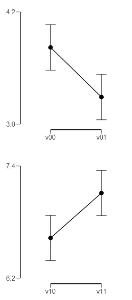
215
Figure 44. Means per condition with associated 95% Bayesian credible intervals.
Figure 45 and Figure 46 provide a visual synopsis the most essential results of the
Bayesian analysis in a concise format: 1) a visualisation the prior distribution of the
effect sizes, 2) the associated posterior distributions, 3) the associated 95% Bayesian
credible intervals, 4) the posterior medians, 5) the Bayes Factors, 6) the associated
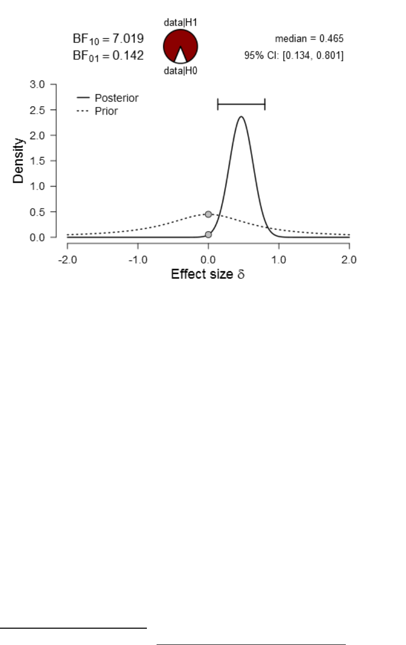

217
Figure 46. Prior and posterior plot for the difference between V
10
vs. V
11
.
In order to establish the robustness of our findings (i.e., their independence from
specific priors), we performed Bayes Factor robustness checks for various Cauchy
priors per comparison. The results indicated that the outcome was reasonably stable
under various parametrisations of the Cauchy priors. For the first comparison (V
00
vs.
V
01
) the maximum Bayes Factor was obtained at r ≈ 0.29 (max BF
10
≈ 9.37). For the
second comparison (V
10
vs. V
11
) the maximum evidence in favour of H
1
was associated
with r ≈ 0.27 (max BF
10
≈ 7.68). Details of the BF robustness analysis are provided in
Figure 47 and Figure 48, respectively.
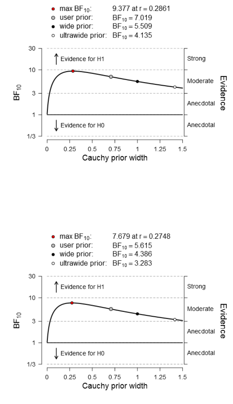
218
Figure 47. Bayes Factor robustness check for condition V
00
vs. V
10
using various
Cauchy priors.
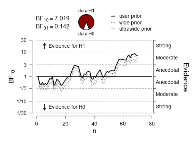
219
Figure 48. Bayes Factor robustness check for condition V
01
vs. V
11
using various
Cauchy priors.
Similar to the analysis reported in Experiment 1, we performed a sequential Bayes
Factor analysis to examine the accumulation of evidence in favour of H
1
as a function of
the number of data points/participants. The results of this analysis are visualised in
Figure 49 and Figure 50.
Figure 49. Sequential analysis depicting the accumulation of evidence as n accumulates
over time (for experimental condition V
00
vs. V
10
).

220
Figure 50. Sequential analysis depicting the accumulation of evidence as n accumulates
over time (for experimental condition V
00
vs. V
10
).
In sum, the Bayes Factor analysis corroborated our initial hypotheses and provided an
analytic cross-validation of the preceding frequentist analysis. We demonstrated the
robustness of our finding under various priors and we investigated the accrual of
evidence as a function of time (viz., as a function of the number of participants). The
Bayes Factor provided a quantitative metric for the “strength of evidence” which was
unavailable in the frequentist framework. In addition, the results of the analysis can be
utilised for future research in the sense of Dennis Lindley’s motto: “Today's posterior is
tomorrow's prior” (Lindley, 1972), or as Richard Feynman put it “Yesterday's sensation
is today's calibration” to which Valentine Telegdi added“...and tomorrow's
background”. In the long run, this incremental (subjective) Bayesian philosophy of
science thus facilitates the cumulative (quasi-evolutionary) progress of science because
221
it enables the explicit integration of prior knowledge. This is a huge advantage over
NHST. The importance of this generic argument cannot be overstated.
222
3.4.3 Bayesian parameter estimation using Markov chain
Monte Carlo methods
This section reports the application Bayesian parameter estimation via Markov chain
Monte Carlo (MCMC) methods. We utilised the same hierarchical Bayesian model as
described in Experiment 1. That is, we specified the same priors on all parameters and
performed the simulation with the same specifications. As in the previous analysis, we
performed the MCMC simulation with 100000 iterations, 500 adaptation steps, and
1000 burn-in steps (no thinning, 3 Markov chains in parallel). We will first report the
convergence diagnostics and we will then proceed to examine the posterior
distributions.
3.4.3.1 MCMC simulation output analysis and convergence diagnostics
The converge diagnostics indicated that the Markov Chain reached the steady-state
(equilibrium) distribution π.
(the potential scale reduction factor) had a value of 1,
indicating that the chain reached its equilibrium distribution and the ESS (effective
sample size) had an acceptable value (i.e., smaller than 100000). On this basis we
proceeded with the analysis and examined the posterior distribution. Exact diagnostic
metrics are provided in Table 16. Detailed visual and numerical diagnostics are attached
in Appendix C4.

223
Table 16
MCMC convergence diagnostics based on 100002 simulations for the difference in
means between experimental condition V
00
vs. V
10
.
Iterations = 601:33934
Thinning interval = 1
Number of chains = 3
Sample size per chain = 33334
mean sd mcmc_se n_eff Rhat
mu_diff 0.524 0.183 0.001 62608 1
sigma_diff 1.467 0.143 0.001 46091 1
nu 37.878 30.016 0.209 20702 1
eff_size 0.360 0.129 0.001 63638 1
diff_pred 0.527 1.573 0.005 99385 1
Model parameters:
• μ
∆
(mu_diff): The mean pairwise difference between experimental conditions
• σ
∆
(sigma_diff): the scale of the pairwise difference (a consistent estimate of SD
when nu is large)
• ν (nu): The degrees-of-freedom for the bivariate t distribution fitted to the
pairwise difference
• δ (eff_size): the effect size calculated as (
0)/
.
• μ
∆pred
(diff_pred): predicted distribution for a new datapoint generated as the
pairwise difference between experimental conditions

224
Convergence diagnostics:
• mcmc_se (Monte Carlo Standard Error, MCSE): The estimated standard error of
the MCMC approximation of the mean.
• n_eff (Effective Sample Size, ESS): A crude measure of effective MCMC
sample size.
• Rhat (Shrink factor,
): the potential scale reduction factor (at convergence,
1).
3.4.3.2 Bayesian parameter estimation for the difference between
experimental condition V
00
vs. V
10
The posterior predictive plot indicated a good model fit (illustrated in Figure 51). The
estimated mean difference between experimental condition V
00
vs. V
10
was μ
∆
≈ 0.52
with a 95% HDI ranging from [-0.17, -0.89]. The associated effect size was estimated to
be δ ≈ 0.36 and the associated 95% HDI spanned [0.11 -0.61]. The standard deviation of
the difference was estimated to be σ
∆
≈ 1.47. We utilised the 95% HDI in combination
with a predefined ROPE in order draw inferences concerning our a priori hypothesis.
The ROPE for the means difference and the effect size did not overlap with 95% HDI.
Based on the previously discussed ROPE/HDI decision algorithm (Kruschke, 2014), we
concluded that H
0
can be rejected and H
1
accepted. A numerical summary of the
results
141
is given in Table 17 and a comprehensive visual synopsis is provided in
Figure 51. In sum, the analysis reconfirmed our previous statistical inference and lends
further support to our conclusions. Moreover, we obtain precise parameter estimates
141
Note: The reported posterior parameter estimates might vary slightly because they are based on a
different MCMC chains and therefore influenced by the randomness in the MCMC chains. We ran the
same analyses several times to establish the robustness of the parameter estimates across MCMC samples.

225
with associated high-density intervals which were unavailable in the previous
analyses.
142
Table 17
MCMC results for Bayesian parameter estimation analysis based on 100002
simulations for the difference in means between experimental condition V
00
vs. V
10
.
mean sd HDIlo HDIup %<comp %>comp
mu_diff 0.523 0.183 0.169 0.886 0.002 0.998
sigma_diff 1.467 0.143 1.199 1.762 0.000 1.000
nu 37.892 30.417 2.661 98.663 0.000 1.000
eff_size 0.360 0.129 0.110 0.613 0.002 0.998
diff_pred 0.533 1.571 -2.664 3.563 0.359 0.641
Note. 'HDIlo' and 'HDIup' are the limits of a 95% HDI credible interval.
'%<comp' and '%>comp' are the probabilities of the respective parameter being smaller
or larger than 0.
142
Based on the richness of information supplied by the MCMC based Bayesian parameter estimation
approach, we argue that this statistical inferential technique is by a large margin superior to NHST and
Bayes Factor analysis (Kruschke & Liddell, 2015, 2017a; Kruschke & Vanpaemel, 2015).
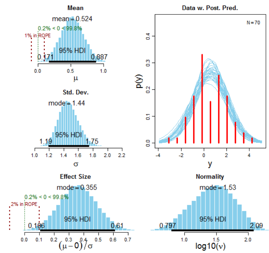
226
Figure 51. Comprehensive summary of the Bayesian parameter estimation.
Left panel: Posterior distribution of the difference between means (experimental
condition V
00
vs. V
10
) with associated 95% high density credible intervals and ROPE [-
0.1,0.1], the standard deviation of the estimated difference and the corresponding effect
size δ with its associated ROPE ranging from [-0.1,0.1] and 95% HDI.
Right panel: Posterior predictive plot (n=30) for the mean difference. The normality
parameter log
10
(ν) with accompanying 95% HDI.

227
3.4.3.3 Bayesian parameter estimation for the difference between
experimental condition V
01
vs. V
11
The convergence diagnostics (Table 18, see Appendix C5 for additional details)
indicated that the MCMC samples converged to the equilibrium distribution and we
proceeded with the inspection of the posterior distributions.
Table 18
MCMC convergence diagnostics based on 100002 simulations for the difference in
means between experimental condition V
00
vs. V
10
.
Iterations = 601:33934
Thinning interval = 1
Number of chains = 3
Sample size per chain = 33334
mean sd mcmc_se n_eff Rhat
mu_diff -0.485 0.170 0.001 60960 1
sigma_diff 1.358 0.136 0.001 41291 1
nu 35.160 28.789 0.208 19274 1
eff_size -0.361 0.130 0.001 57623 1
diff_pred -0.488 1.454 0.005 98609 1
As can be seen in Figure 52, the posterior predictive plot indicated a good
approximation of the empirical data. The estimated mean difference between
experimental condition V
01
vs. V
11
was μ
∆
≈ -0.48, 95% HDI [-0.82, -0.15]. The effect
size was δ ≈ -0.36 and the associated 95% HDI ranged from [-0.62 -0.10]. The standard
deviation of the difference was σ
∆
≈ 1.36, 95% HDI [1.10, 1.63]. The difference
between means was credible and the ROPE [-0.1, 0.1] for the difference in means and
the corresponding effect size did not overlap with 95% HDI. We thus rejected H
0
and

228
accepted H
1
. A quantitative overview of the results is given in Table 19 and Figure 52
provides a comprehensive visual summary. Taken together, the analysis corroborated
our previous analyses and strengthened the credibility of our a priori hypotheses from a
Bayesian point of view.
Table 19
MCMC results for Bayesian parameter estimation analysis based on 100002
simulations for the difference in means between experimental condition V
01
vs. V
11
.
mean sd HDIlo HDIup %<comp %>comp
mu_diff -0.485 0.171 -0.817 -0.143 0.998 0.002
sigma_diff 1.358 0.137 1.096 1.634 0.000 1.000
nu 35.134 28.790 2.405 93.144 0.000 1.000
eff_size -0.361 0.131 -0.618 -0.103 0.998 0.002
diff_pred -0.485 1.461 -3.373 2.404 0.635 0.365
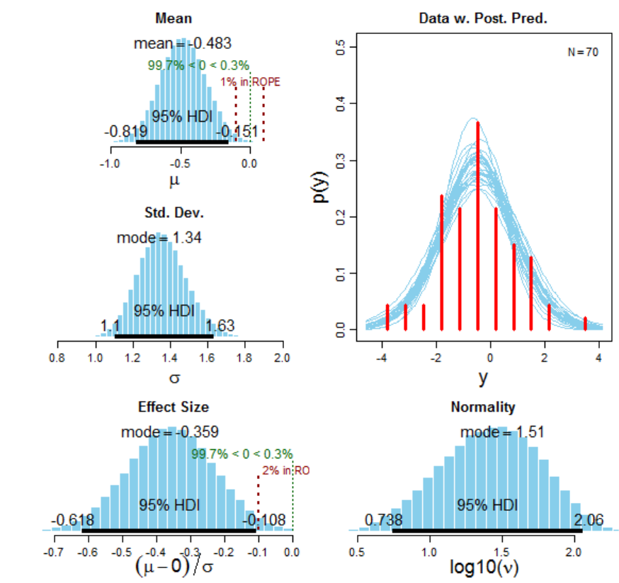
229
Figure 52. Visual synopsis of the results of the Bayesian parameter estimation.
Left panel: Posterior distribution of the difference between means (experimental
condition V
01
vs. V
11
) with associated 95% high density credible intervals, and ROPE [-
0.1,0.1],the standard deviation, of the estimated difference and the corresponding effect
size. Right panel: Posterior predictive plot (n=30) for the mean difference. The
normality parameter log
10
(ν) with accompanying 95% HDI.
In sum, we concluded that the differences of means between experimental conditions
V
00
vs. V
01
and V
10
vs. V
11
are credible. That is, both pairwise comparisons resulted in
values that were credibly different from zero. Hence, we rejected H
0
for both
230
hypotheses. The conclusion is motivated by the nonoverlapping position of the 95%
equal-tail high density credible interval relative to the region of practical equivalence.
This inference is congruent with the conclusion based on the previous frequentists
NHST analysis and the Bayes Factor analysis. In addition, we performed a correlation
analysis by computing a classical Pearson's product-moment correlation coefficient and
a Bayesian MCMC based alternative. The results of this supplementary analysis are
attached in Appendix C7.
3.5 Discussion
In conclusion, our results indicate that psychophysical measurements play a
constructive role in perceptual processes. Moreover, our findings are in line with those
reported in the domain of attitudinal judgments (White et al., 2015, 2014b). Our
investigation can be regarded as a psychophysical analogon of the measurement
problem in quantum physics (discussed in more detail in a subsequent chapter). In
quantum physics, it is a well-replicated finding that the mere act taking a measurement
changes the process under investigation. That is, the evolution of the system under
investigation, be it physical or cognitive, is conditional on observation (e.g.,
einselection/wave-function collapse). The constructive role of measurements is
incongruent with classical (deterministic) Markov models which assume that the system
under investigation is always in a fixed and discrete ontological state (even though the
exact state might be unknown, e.g., as postulated various hidden-variable accounts).
An important question concerns the exact definition (operationalisation) of what
constitutes a psychophysical measurement. It is entirely possible that participants make
covert judgments in trails where no response is rquired. We cannot rule out this
231
possibility due to the methodological impossibility to directly access introspective
cognitive states. Such implicit judgment might take place below the threshold of
conscious awareness and participants themselves might therefore be unable to report on
such automatic processes. Only neuroimaging studies would be able to resolve this
question. Using an appropriate experimental design on could subbstract the neuronal
activity associated with conditions in which one expects unconscious judgments from a
baseline level of activity in order to gain insight into this aspect of information
processing. In addition, one could use electromyography in order measure minute
movements at the muscular level (e.g., at the muscle tissue of the hand or fingers).
Moreover, it is likely that EEG measurments could pick up preparatory action potentials
at the level of the premotor cortex long before an actual motor response is emitted. In an
ideal case one would combine EEG and fMRI techniques in order to tobtain a more
complete picture (EEG has a temporal resolution and a low spatial resolution; the
opposite holds true for fMRI). By coupling the signals obtained from the two modalities
one could then draw joint inferences about the underlying cognitive (unconscious)
mechanisms. (In addition, acquiring simultaneous EEG and functional MRI would have
several methodological advantges as potential confounds would be balanced out,
thereby increasing the reliability and validity of the measurements.)
However, even if partcipants engaged in such unconscious judgments there would be a
difference between explicit and implicit modes of responding.
Another question worth discussing concern the question of the level at which
constructive inference takes place. It could be cogently argued that measurment effects
could in principle be prent across the whole experiment. This is an interesting line of
though and it relevant from a complex systems perspective in which one assumes that
principles at the micro scale of the system (e.g., an individual experimental trial) are
232
scale-invariant and are conseuqntly reflected at the macro level of the system (e.g., the
entire experiment). We are in no position to answer this question conclusively (due to a
lack of relevant data). However, this line of thought might even turn out to be relevant
for the acute replication crisis science is currently facing. If a scientific experiment as a
whole constitutes a measurment one could argue that the order in which experiments are
conducted matters (due to constructive interference). This is a sensible idea which
deserves further investigation. Currently, science assumes that replication is
independent of the order in which experiments are conducted. However, this assumption
might not stand the empirical test.
More generally the important questionof what exactly constitutes a measurment is
analogous to adamantine “measurement problem” in quantum physics which is matter
of intense debate in the physics community. We will address this operationalsiational
problem in more detail in the general discussion (§ 6.3.2). At this point it is sufficient to
note that an exact definition is currently unavailable and that there is no consensus in
the scientific community.
CHAPTER 4. EXPERIMENT #3:
NONCOMMUTATIVITY IN SEQUENTIAL
AUDITORY PERCEPTUAL JUDGMENTS
4.1 Experimental purpose
Based on the results of our previous experiments, we were interested whether the
observed effects would be generalisable to another percepetual information processing
modality. Therefore, we designed an audiometric psychophysics experiment which was

233
structurally isomorphic to Experiment 1. Thus, Experiment 3 can be regarded as an
effort to cross-validate and generalise our previously obtained empirical results.
Furthermore, Experiment 3 is a conceptual replication in an effort to establish the
robustness of the previous results. Instead of focusing on the perception of luminance as
we did in the previously reported experiments, we focused on the subjective perception
of loudness (its objectively quantifiable physical equivalent being sound intensity).
Much of the impetus for the current psychoacoustics experiment was derived from the
pertinent quantum cognition literature which suggests that noncommutativity effects in
psychological observables are ubiquitous in many domains of human (and possibly
animal
143
) cognition (Atmanspacher, 2014a, 2016; Atmanspacher & Römer, 2012; Z.
Wang et al., 2013). Our line of reasoning was as follows: If the same effects as observed
in the visual domain in Experiment 1 can be replicated in a different modality of
information processing, then we can be more confident that the noncommutativity
principle is a general and fundamental property of human perception and cognition.
This argument is based on an analogy to computational processes at the neuronal level.
Neurons utilise the same neuronal representations and computational principles across
modalities, that is, there is no difference between the electrochemical computation
principles employed for visual and auditory perception (and all other sensory
modalities). That is, the neural code is identical across information processing
modalities and across species (Bialek, Rieke, de Ruyter van Steveninck, & Warland,
143
An investigation of noncommutativity effects in animal perception would provide another powerful
cross-validation for the general framework of quantum-like noncommutativity effects in cognitive
processes. However, we a not aware that such research has been conducted yet. We would be very
interested in studies examining perceptual noncommutativity in non-human primates. The next step
further down in the phylogenetics hierarchy would be to investigate those processes, for instance, in
bacteria e.g., noncommutativity effects in phototaxis, chemotaxis, and magnetotaxis (Frankel &
Bazylinski, 1994; Gest, 1995; Vladimirov & Sourjik, 2009). If perceptual noncommutativity could be
demonstrated across different taxa (in addition to different sensory modalities) this provide very strong
converging evidence for the generalisability of this principle, viz., scientific consilience (E. O. Wilson,
1998a, 1998b) via methodological polyangulation at multiple levels of biology.
234
1991; Stanley, 2013). It is thus reasonable to argue that perceptual mechanism follow
similar generalisable principles which are modality-unspecific. The current experiment
was thus designed to investigate the modality-nonspecificity of noncommutativity
effects in a controlled experimental fashion which is directly comparable (i.e., empirical
commensurable) to Experiment 1.
4.2 A priori hypotheses
Our a priori hypotheses were isomorphic to those formulated in Experiment 1. We
focused specifically on noncommutativity effects in auditory perceptual judgments.
H
1
: Measuring the intensity of a high loudness stimuli first results in a decrease in the
subsequent judgment for low stimuli as compared to the reverse order.
H
2
: Measuring the perceived loudness of the low loudness stimuli first results in an
increase in the subsequent judgment relative to reverse order.
In symbolic form expressed as follows:
H
: AB BA
where
A = high intensity auditory stimuli
B
= low intensity auditory stimuli

235
4.3 Method
4.3.1 Participants and Design
The experiment was carried out in the psychology laboratory of the University of
Plymouth and ethical approval was obtained from the universities human research ethics
committee. We recruited participants from the general public using web-based
advertising using the Sona participant management software (Sona Experiment
Management System®, Ltd., Tallinn, Estonia; http://www.sona-systems.com) which is
hosted on the universities webserver. In total, 80 participants participated in the
experiment (45 women and 35 men, ages ranging between 18 and 62 years, M
age
=
26.73; SD
age
= 7.17).
4.3.2 Apparatus and materials
As in the previous experiments, we utilised the Python (Python Software Foundation,
2013) based software PsychoPy (J. W. Peirce, 2007, 2008) for the creation of the
experiment. Auditory stimuli were specified by using the “sound component”
144
in
PsychoPy which is based on the “Pyo” audio library (a Python module written in C to
assist digital signal processing script creation)
145
. We created two auditory stimuli
(pure
tones, 400Hz) with varying intensity levels, i.e., we fixed the “loudness” parameter in
PsychoPy to “0.6” and “0.8”, respectively. Recordings of the auditory stimuli can be
downloaded from the following URLs in the “waveform audio file” (*.wav) format:
144
Details can be found under the following URL:
http://www.psychopy.org/builder/components/sound.html
145
http://ajaxsoundstudio.com/pyodoc/

236
http://irrational-decisions.com/phd-thesis/auditory-stimuli/stimulus-0.6.wav
http://irrational-decisions.com/phd-thesis/auditory-stimuli/stimulus-0.8.wav
The complete source code of the experiment can be downloaded from the following
URL as a compressed ZIP archive: http://irrational-decisions.com/?page_id=618
4.3.3 Experimental Design
The structure of the experiment was a repeated measures design consisting of auditory
stimuli with different intensity levels. The presentation of stimuli was randomly
alternated in order to investigate sequential noncommutativity effects in auditory
perceptual. As in Experiment 1, we utilised a fully counterbalanced Latin-square design
and the experimental conditions were thus as follows.
Variable declarations for experimental conditions:
V
00
= low intensity → low intensity
V
01
= low intensity → high intensity
V
11
= high intensity → high intensity
V
10
= high intensity → low intensity
4.3.3.1 Procedure
Before the commencement of the study, participants were briefed and accorded written
informed consent. Subsequently, participants were seated in front of a PC equipped with
headphones and received further instructions.
237
4.3.4 Sequential auditory perception paradigm
The entire experimental paradigm was isomorphic with respect to Experiment 1 in order
to ensure commensurability between experimental results. The only difference was that
we switched the perceptual modality from visual perception to auditory perception in
order investigate the generalisability/modality-nonspecificity of our prior experimental
findings.
4.4 Statistical Analysis
We applied the same statistical analyses as detailed in Experiment 1. However, for
reasons of brevity, we did not perform nonparametric and Bayesian bootstraps (the
results converged in our previous analyses). We first conducted a frequentist analysis
using parametric and non-parametric techniques. We then performed a Bayes Factor
analysis to get a more accurate probabilistic picture of the credibility of the results.
Finally, we utilised much more flexible Bayesian parameter estimation techniques using
Markov Chain Monte Carlo methods to obtain precise estimates of the relevant
parameters. In the later analytical framework, decision concerning our a priori
hypotheses were again based on the previously discussed ROPE/HDI algorithm
(thereby engaging the engaged reader to construct her own idiosyncratic decision
criteria by constructing a ROPEs with varying radii).
Frequentist analysis
We first examined the distributional properties of the dataset. Descriptive statistics are
provided in Table 1. The Shapiro-Wilk’s W test indicated that the data did satisfy the

239
Table 21). We also performed the Kolmogorov-Smirnov test, although simulations
studies indicate that Shapiro-Wilk test should generally preferred (Razali & Wah,
2011). All formal tests of Gaussianity indicated that parametric testing procedures are
appropriate for the data at hand. However, quantitative p-value based test of Gaussianity
are imperfect and visual inspection via Q-Q plots is generally recommended (see
Appendix D for Q-Q plots and additional test results, e.g., the Cramér–von Mises
criterion). Visual inspection reconfirmed that the distributional assumptions were
satisfied, and we proceeded with parametric testing.
We performed two paired samples t-test (i.e., repeated measures t-test, two-tailed) to
evaluate our hypotheses.
Table 20
Descriptive statistic for experimental conditions.
N
Mean
SD
SE
v00
80
2.528
0.995
0.111
v10
80
3.100
1.060
0.119
v01
80
6.590
1.020
0.114
v11
80
6.030
1.030
0.115

240
Table 21
Shapiro-Wilk’s W test of Gaussianity.
W
p
v00
-
v10
0.992
0.881
v01
-
v11
0.984
0.409
Note. Significant results suggest a deviation from normality.
4.4.1 Parametric paired samples t-tests
The results of both t-test (Gosset, 1908) indicated that the differences between sample
means were statistically significant at the conventional arbitrary α-level (R. Fisher,
1956). The t-tests indicated that low intensity auditory stimuli were on average rated
significantly lower in loudness when anteceded by equivalent stimuli (V
00
; M=2.53,
SD=1.00) as compared to low intensity stimuli which were anteceded by high intensity
stimuli (V
10
; M=3.10, SD=1.06), M
Δ
=-0.57; t(79)=-3.38, p=0.001, 95%CI [-0.91, -0.24];
Cohen’s d=-0.38,
A visual representation of the results is provided in
146
95%CI
for d [-0.60, -0.15].
By contrast, the loudness of high intensity auditory stimuli were on average rated
significantly higher when they were anteceded by low intensity stimuli (V
01,
M=6.59,
SD=1.02) relative to high intensity stimuli anteceded by equivalent stimuli (V
11
,
M=6.03, SD=1.03), M
Δ
=0.56; t(79)=3.44, p<0.001, 95%CI [0.24, 0.88]; Cohen’s d=-
0.38, 95%CI for d [0.16, 0.60].
Figure 53 and a detailed summary is given in Table 23.
146
Effect sizes were calculated based on the formula described by Moors (2011):
=
where the pooled standard deviation (s) is defined as =
(
)
(
)

241
Furthermore, we computed various alternative statistics (e.g., the Vovk-Sellke
Maximum p-Ratio, VS-MPR). A numerical summary is provided in Table 3. In
addition, a comprehensive summary of the complete results is provided under the
following URL:
http://irrational-decisions.com/phd-thesis/exp3/results-exp3.html
The pattern of results was congruent with those obtained in Experiment 1 and confirmed
our a priori hypotheses. In other terms, the results provided a cross-validation of our
previous findings and support the generalisability of our findings across perceptual
modalities. We followed-up with a Bayes Factor analysis which is a much more
powerful analytic procedure which circumvents the well-documented logical flaws
associated with frequentist NHST.
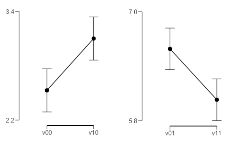
242
Figure 53. Visualisation of differences in means between conditions with associated
95% confidence intervals.

243
Table 22
Paired samples t-test and nonparametric Wilcoxon signed-rank tests
95% CI for Location
Parameter
95% CI for
Effect Size
Test
Statistic
df
p
VS-
MPR*
Location
Parameter
SE
Difference
Lower
Upper
Effect
Size
Lower
Upper
v00
-
v10
Student
-3.379
79
0.001
47.928
-0.572
0.169
-0.909
-0.235
-0.378
-0.604
-0.150
Wilcoxon
976.000
0.002
29.280
-0.560
-0.894
-0.218
-0.398
-0.587
-0.167
v01
-
v11
Student
3.438
79
9.382e -
4
56.247
0.560
0.163
0.236
0.884
0.384
0.156
0.610
Wilcoxon
2299.000
0.001
47.733
0.626
0.286
0.944
0.419
0.192
0.604
* Vovk-Sellke Maximum p -Ratio: Based on the p -value, the maximum possible odds in favor of H over H equals 1/(-e p log( p ))
for p ≤ .37 (Sellke, Bayarri, & Berger, 2001).
Note. For the Student t-test, location parameter is given by mean difference d ; for the Wilcoxon test, effect size is given by the
Hodges-Lehmann estimate.
Note. For the Student t-test, effect size is given by Cohen's d ; for the Wilcoxon test, effect size is given by the matched rank biserial
correlation.
244
4.4.2 Bayes Factor analysis
We used the same specification for the Bayesian model as in the previous experiments.
The resulting Bayes Factor for the first pairwise comparison (experimental condition
V
00
vs. V
10
) was BF ≈ 21.64 which can be interpreted as strong evidence for H
1
in
Jeffreys’ heuristic schema. The data is thus approximately 21 times more likely under
H
1
than under H
0
, P(D│H
1
) ≈ 21.64; and its reciprocal is P(D│H
0
) ≈ 0.05. The second
contrast resulted in a BF of ≈ 25.63 which falls in the same category, thereby
indicating that P(D│H
1
) ≈ 25.63; P(D│H
0
) ≈ 0.04. All hypotheses were tested two-
tailed. However, it could be argued that directional one-tailed tests would be
appropriate, given the previously obtained results. In this case the respective Bayes
Factors would be simply multiplied by a factor of two. Therefore, we report results for
one-tailed test which renders the statistics directly commensurable between experiments
and thence across perceptual modalities. Descriptive statistics and the associated
Bayesian 95% Bayesian credible intervals are given in Table 24. In addition, the results
are visualised in Figure 54 and prior and posterior plots are provided in Figure 55 and
Figure 56, respectively. For reasons of brevity, we will not discuss the analysis in
greater detail. Additional information can be found in Appendix D (e.g., Bayes Factor
robustness check for various Cauchy priors, Sequential analysis of the accumulation of
evidence, etc.).
In sum, the results corroborate our previous analysis and indicate probabilistically that
the evidence for H
1
is strong (in Jeffrey’s heuristic interpretational scheme discussed
before). In direct comparison to Experiment 1, both Bayes Factors indicate that the
evidence for noncommutativity is even stronger for auditory perceptual judgments.
Recall that the Bayes Factors for Experiment 1 were BF ≈ 9.20 and BF ≈ 24.82,
respectively.

245
Table 23
Bayes Factors for orthogonal contrasts.
BF
error %
v00
-
v10
21.637
1.616e -7
v01
-
v11
25.629
1.460e -7
Table 24
Descriptive statistics and associated Bayesian 95% credible intervals.
95% Credible Interval
N
Mean
SD
SE
Lower
Upper
v00
80
2.528
0.995
0.111
2.307
2.749
v10
80
3.100
1.060
0.119
2.864
3.336
v01
80
6.590
1.020
0.114
6.363
6.817
v11
80
6.030
1.030
0.115
5.801
6.259
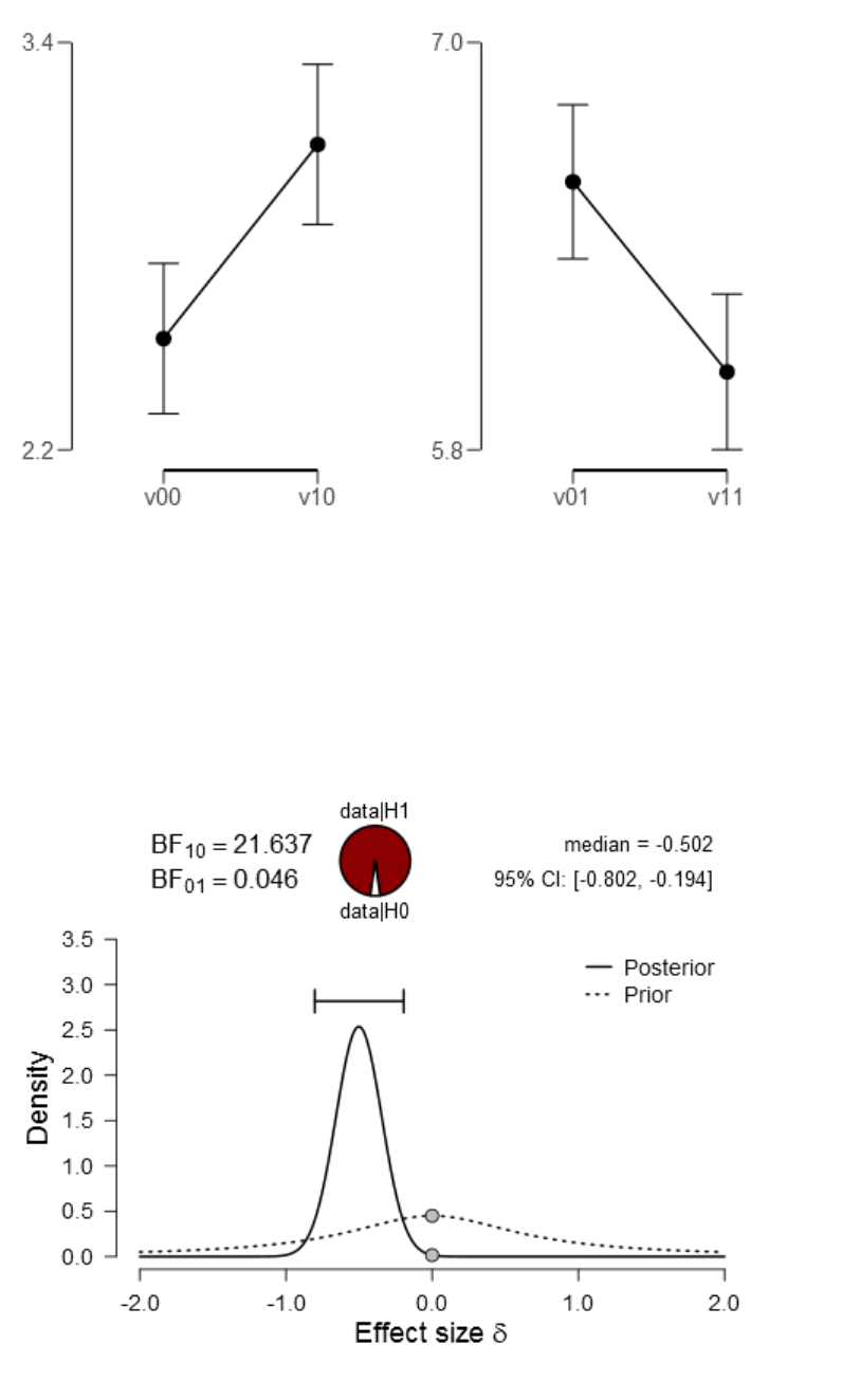
246
Figure 54. Difference between means per condition with associated 95% Bayesian
credible intervals.
Figure 55. Prior and posterior plot for the difference between V
00
vs. V
10
.

247
Figure 56. Prior and posterior plot for the difference between V
01
vs. V
11
.
We then followed-up the Bayes Factor analysis with a Bayesian parameter estimation
procedure using MCMC methods in order to obtain precise posterior intervals. The BPE
approach allows draw sensible inferences based on the previously discussed HDI/ROPE
algorithm. The statistical inferential decisions based on Bayesian parameter estimation
and Bayes Factor analysis do not necessarily converge, that is, they can lead to different
conclusions.
248
4.4.3 Bayesian a posteriori parameter estimation using
Markov chain Monte Carlo methods
As in in the previously reported experiments, we utilised Bayesian parameter estimation
techniques based on MCMC simulation methods to obtain precise estimates of θ,.
Specifically, the primary desideratum of this analysis was to obtain an accurate estimate
of posterior characteristics, i.e., (
,
,
,
, |). The numerous significant
advantages of this approach have been adumbrated in the previous chapters. We utilised
the exact same model as specified in Experiment 1. Therefore, we will skip the detailed
model specifications and immediately present the results in the following subsections,
starting with the convergence diagnostics which evaluate whether the stationary
equilibrium distribution π of the Markov Chain had been reached by our computations.
4.4.3.1 MCMC analysis and convergence diagnostics
The convergence diagnostics indicated that the equilibrium distribution π had been
reached. A summary is provided in Appendix C4and we refer to Experiment 1 for an
explanation of the various diagnostic criteria. Detailed convergence diagnostics for all
parameters can be found in Appendix D. We thus proceeded with the analysis of the
posterior distribution which is reported in the following subsection.
(Rhat, the
potential scale reduction factor) had a value of 1, indicating that the chain reached π.

249
4.4.3.2 Markov chain Monte Carlo simulation output analysis and
convergence diagnostics for experimental conditions V
00
and
V
10
After fitting our model, using the Bayesian parameter approach, we obtained a
distribution of credible values the pertinent parameters. A numerical summary is given
in Table 25 and a comprehensive synopsis is given in Figure 57.
Table 25
Numerical summary of the Bayesian parameter estimation for the difference between
means for experimental condition V
00
vs. V
10
with associated 95% posterior high density
credible intervals.
mean median mode HDI% HDIlo HDIup compVal %>compVal
mu -0.564 -0.564 -0.557 95 -0.908 -0.231 0 0.079
sigma 1.483 1.477 1.458 95 1.226 1.750
nu 39.002 30.709 15.903 95 2.794 98.714
log10nu 1.473 1.487 1.509 95 0.815 2.080
effSz -0.384 -0.383 -0.389 95 -0.624 -0.151 0 0.079
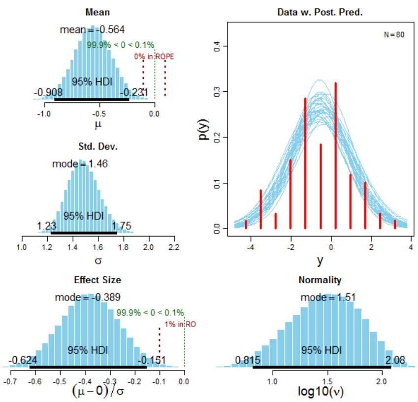
250
Figure 57. Visual summary of the Bayesian parameter estimation for the difference
between means for experimental condition V
00
vs. V
01
with associated 95% HDIs and a
ROPEs ranging from [-0.1, 0.1].
Left panel: Posterior distribution of the difference between means with associated 95%
high density credible intervals and ROPE [-0.1,0.1], the standard deviation of the
estimated difference and the corresponding effect size δ with its associated ROPE
ranging from [-0.1,0.1] and 95% HDI. Right panel: Posterior predictive plot (n=30) for
the mean difference. The normality parameter log
10
(ν) with accompanying 95% HDI.

251
4.4.3.3 Markov chain Monte Carlo simulation output analysis and
convergence diagnostics for experimental conditions V
01
and
V
11
Table 26 summarises the convergence diagnostics and the results for the second
pairwise comparison (V
01
and V
11
) are given in Table 27. A complete summary of the
analysis is provided in Figure 58.
Table 26
MCMC convergence diagnostics based on 100002 simulations for the difference in
means between experimental condition V
01
vs. V
11
.
Rhat n.eff
mu 1.000 61128
nu 1.001 18842
sigma 1.000 38649
Table 27
Numerical summary of the Bayesian parameter estimation for the difference between
means for experimental condition V
01
vs. V
11
with associated 95% posterior high density
credible intervals.
mean median mode HDI% HDIlo HDIup compVal %>compVal
mu 0.577 0.577 0.564 95 0.248 0.901 0 100
sigma 1.414 1.409 1.404 95 1.158 1.682
nu 36.293 27.759 13.043 95 2.652 94.768
log10nu 1.429 1.443 1.484 95 0.757 2.072
effSz 0.412 0.410 0.411 95 0.167 0.664 0 100
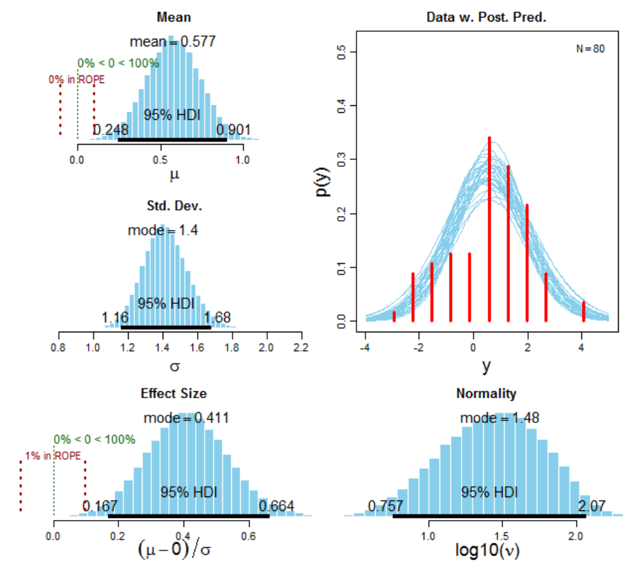
252
Figure 58. Visual summary of the Bayesian parameter estimation for the difference
between means for experimental condition V
10
vs. V
11
with associated 95% HDIs and a
ROPEs ranging from [-0.1, 0.1]. Left panel: Posterior distribution of the difference
between means with associated 95% high density credible intervals and ROPE [-
0.1,0.1], the standard deviation of the estimated difference and the corresponding effect
size δ with its associated ROPE ranging from [-0.1,0.1] and 95% HDI. Right panel:
Posterior predictive plot (n=30) for the mean difference. The normality parameter
log
10
(ν) with accompanying 95% HDI.
253
4.5 Discussion
The results of this experiment replicated the findings of Experiment 1 and thereby
supported the modality-nonspecificity and generalisability of our results. That is, the
findings confirmed our a priori predictions and demonstrate noncommutativity effects
in psychophysical auditory judgments similar to those found in the visual domain.
Moreover, the results of the statistical analyses are in line with the general predictions
formulated by Atmanspacher and colleagues (Atmanspacher, 2014, 2016;
Atmanspacher & Römer, 2012b). The implications of these empirical results will be
discussed in a broader context in the general discussion section.
254
CHAPTER 5. EXPERIMENT #4:
CONSTRUCTIVE MEASUREMENT EFFECTS
IN SEQUENTIAL AUDITORY PERCEPTUAL
JUDGMENTS
5.1 Experimental purpose
The primary purpose of this experiment was to cross-validate the empirical findings
obtained in Experiment 2 in a different sensory modality in order to establish the
generalisability (i.e., modality-nonspecificity) of the results obtained in Experiment 2.
Therefore, the experimental designs were isomorphic with the exception that auditory
stimuli were used instead of visual stimuli. The methodological correspondence
between experiments thus enabled direct comparability of results (i.e., empirical
commensurability).
5.2 A priori hypotheses
The hypotheses were identical to those formulated in Experiment 2 and were likewise in
accordance with predictions derived from the relevant quantum cognition literature
(Atmanspacher, 2014a, 2016; Atmanspacher & Römer, 2012; Z. Wang et al., 2013).
H
1
: Measuring subjectively perceived loudness of the high intensity auditory stimuli
first (i.e., binary measurement condition) results in a decrease in the subsequent
judgment for the low intensity stimuli as compared to the opposite order.
H
2
: Measuring the loudness of the low intensity auditory stimuli first results in an
increase in the subsequent judgment relative to opposite order.
255
In symbolic form the null and alternative hypotheses are expressed as follows:
In symbolic form expressed as follows:
H
:
>
H
:
<
where
V
00
= high intensity stimuli → low intensity stimuli (singular measurement)
V
01
= high intensity stimuli → low intensity stimuli (binary measurement)
V
10
= low intensity stimuli → high intensity stimuli (singular measurement)
V
11
= low intensity stimuli → high intensity stimuli (binary measurement)
The main goal of this audiometric psychophysics experiment was thus to investigate the
constructive influence of an intermediate introspective psychophysical judgement on a
subsequent one. As pointed out before, the constructive role of measurements is pivotal
to the basic tenets of quantum mechanics and similar effects have been documented in
various cognitive domains (e.g., Pothos & Busemeyer, 2013).
5.3 Method
5.3.1 Participants and Design
The experiment was conducted in the computer laboratory at Manipal University Jaipur
in India. Ethical approval was obtained from the head of the Department of Psychology,
Professor Geetika Tankha who supervised this study.

256
One hundred undergraduate students participated in this study (62 women and 38 men,
ages ranging between 18 and 25 years, M
age
= 19.91; SD
age
= 2.35). Students were
recruited via email and flyers which were distributed on campus. As in the previous
experiments, a custom-made website was designed in HTML was utilised to advertise
the study in an attractive way to the student population. All participants were financially
reimbursed for their participation (₹800)
148
.
5.3.2 Apparatus and materials
We utilised the same stimuli as in Experiment 2 for this audiometric experiment, i.e.,
two auditory stimuli of the same frequency but with varying intensity levels (for details
see the methods section of Experiment 2).
As in Experiment 2, the entire experiment was implemented in PsychoPy. The
associated Python source-code can be accessed under the following URL as a
compressed ZIP archive: http://irrational-decisions.com/?page_id=618
5.3.3 Experimental Design
The structure of the experiment was a 2(measurement condition: singular rating vs.
binary measurement) x 2(stimulus order: high intensity → low intensity vs. low
intensity → high intensity) repeated measures design. The dependent measure was the
condition dependent intensity rating which was recorded on a VAS as in our previous
experiments.
148
Due to the extremely chaotic demonetization of all ₹500 and ₹1,000 banknotes of the Mahatma
Gandhi Series the payment was delayed for approximately half of the participants. The decision of the
government was unforeseen and caused serious social problems as money became a scarce resource
overnight. It was impossible to withdraw any “new” money from banks for several days which caused an
extremely chaotic situation in the whole country.
257
5.3.4 Procedure
Before the commencement of the study, participants were briefed and accorded
informed consent. Subsequently, participants were seated in front of a personal
computer and received further instructions.
5.3.5 Sequential auditory perception paradigm
The experimental design was identical to Experiment 2 and we refer to the methods
section for details to avoid repetition. The only difference was that we switched the
sensory modality, i.e., we utilised auditory stimuli instead of visual stimuli. A
diagrammatic depiction of the temporal sequence of events within two successive
experimental trials is depicted in Figure 59.
The within-trial sequence of events was as follows: Initially, a white fixation cross was
displayed on a black background until a manual response (single left mouse-click) was
emitted. The following instructions were presented to participants: “New trial: Please
fixate the cross with your eyes and click the mouse when you are ready”. Next, an
auditory stimulus of either high or low intensity was binaurally presented (via
headphones). The stimulus was then replaced by a rating request or no rating request,
(i.e., binary vs. singular measurement condition) which was presented until a response
was emitted (either a rating on the VAS or a mouse-click response, depending on the
respective experimental condition). After that, the second auditory stimulus appeared
for the same temporal duration followed by the final rating request. In sum, participants
completed a total of 600 experimental trials.
Upon completion of the experiment, participants were debriefed and were given the
possibility to ask questions concerning the purpose and theoretical background of the
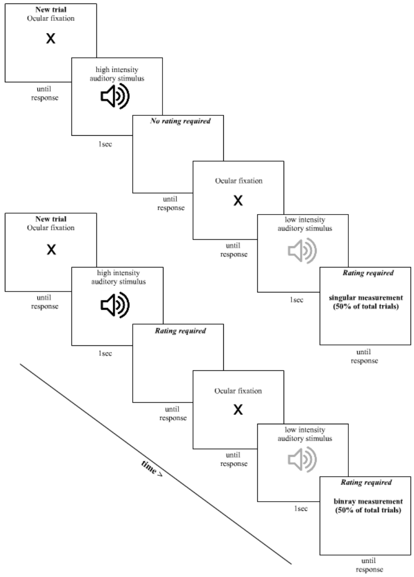
258
study. Finally, participants were thanked for their cognitive efforts, financially
reimbursed, and released.
259
Figure 59. Diagrammatic representation of the temporal sequence of events within two
successive experimental trials in Experiment 4.
5.4 Statistical Analysis
As in the previous statistical analyses, we employed various complementary inferential
techniques to test our predictions. As pointed out before, statistical methods are
currently rapidly evolving. Although still widely used (and taught), NHST has been
conclusively dismantled as a statistical chimera. It is widely misinterpreted by
professional researchers, i.e., more than 80% of statistics lecturers at universities are
unable to interpret the most simple NHST analysis correctly (Haller & Krauss, 2002;
Oakes, 1986). Novel methods have been proposed by the APA (Cumming, 2014) but
they nevertheless do not emphasise the Bayesian alternatives emphatically enough
(Kruschke & Liddell, 2017b). That is, the APA primarily tries to reinforce the usage of
confidence intervals and effect sizes, both of which are ultimately based on frequentist
principles. Furthermore, it has been experimentally demonstrated that confidence
intervals are also widely misinterpreted by the vast majority of professional researchers
in various academic disciplines (Hoekstra, Morey, Rouder, & Wagenmakers, 2014).
Therefore, we utilised Bayesian inferential statistics in addition to the conventional
frequentist methods in our analyses. However, the Bayesian camp is subdivided. While
some argue for the adequacy of the Bayes Factor (Dienes, 2014, 2016; Richard D.
Morey & Rouder, 2011; Rouder, Morey, Verhagen, Swagman, & Wagenmakers, 2017),
other emphasize the numerous advantages which Bayesian parameter estimation based
on Markov Chain Monte Carlo methods has over and above the more straightforward
Bayes Factor analysis (Kruschke, 2014; Kruschke & Liddell, 2015; Kruschke et al.,

260
2017). Therefore, we utilise both approaches in order to cross-validate our statistical
results in different mathematical frameworks.
5.4.1 Frequentist analysis
We first tested the underlying distributional assumption and conducted several tests of
normality (see Appendix E). We then proceeded to test our research hypotheses with a
paired samples t-test (i.e., repeated measures t-test. The associated descriptive statistics
are depicted in Table 28.
Table 28
Descriptive statistics for experimental conditions.
N
Mean
SD
SE
v00
100
4.430
1.090
0.109
v01
100
3.910
1.020
0.102
v10
100
6.900
1.030
0.103
v11
100
7.370
1.070
0.107
Variable declarations:
V
00
= high intensity stimuli → low intensity stimuli (singular measurement)
V
01
= high intensity stimuli → low intensity stimuli (binary measurement)
V
10
= low intensity stimuli → high intensity stimuli (singular measurement)
V
11
= low intensity stimuli → high intensity stimuli (binary measurement)

261
Table 29
Shapiro-Wilk’s W test of Gaussianity.
W
p
v00
-
v01
0.986
0.350
v10
-
v11
0.993
0.896
Note. Significant results suggest a deviation from normality.
The t-test indicated significant differences between conditions. The first comparison
indicated that V
00
was rated significantly higher relative to V
01,
M
Δ
=0.52; t(99)=3.42,
p<0.001, 95%CI [0.22, 0.82]; Cohen’s d=0.34, 95%CI
for d [0.14, 0.54]. Conversely,
V
10
was rated significantly lower as compared to V
11
M
Δ
=-0.47; t(99)=-3.10, p=0.003,
95%CI [-0.77, -0.18]; Cohen’s d=-0.31, 95%CI
for d [-0.51, 0.11]. A comprehensive
tabular summary including the Vovk-Sellke maximum p-ratio (Sellke et al., 2001;
Vovk, 1993) is provided in Table 30. Moreover, the results are visualised in Figure 60
and the distributional properties are depicted in Figure 61.
In sum, the results supported our initial predictions and provided a second conceptual
cross-validation of the findings reported by White, Photos, & Busemeyer (White et al.,
2014b).
A comprehensive synopsis of the results including the Vovk-Sellke maximum p-ratio
(Sellke et al., 2001; Vovk, 1993) is provided under the following URL as a HTML-file:
http://irrational-decisions.com/phd-thesis/frequentist-analysis-exp4.html
In addition we report p
rep
, i.e., the probability of replicating the results upon an exact
replication as introduced by Peter Killeen (2005a) as an alternative to conventional p
values (see Appendix E14).
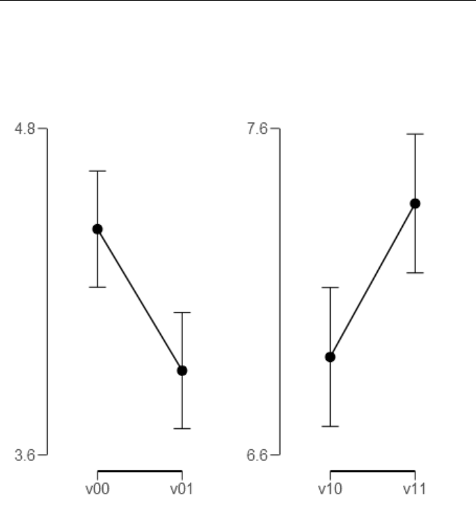
262
A comprehensive summary of the results is provided under the following URL:
http://irrational-decisions.com/phd-thesis/exp2/frequentist_t-test_exp4/
In the next section, we repeated the analysis using Bayesian parameter estimation via
Markov chain Monte Carlo sampling.
Figure 60. Visual summary of differences between means with associated 95%
confidence intervals.
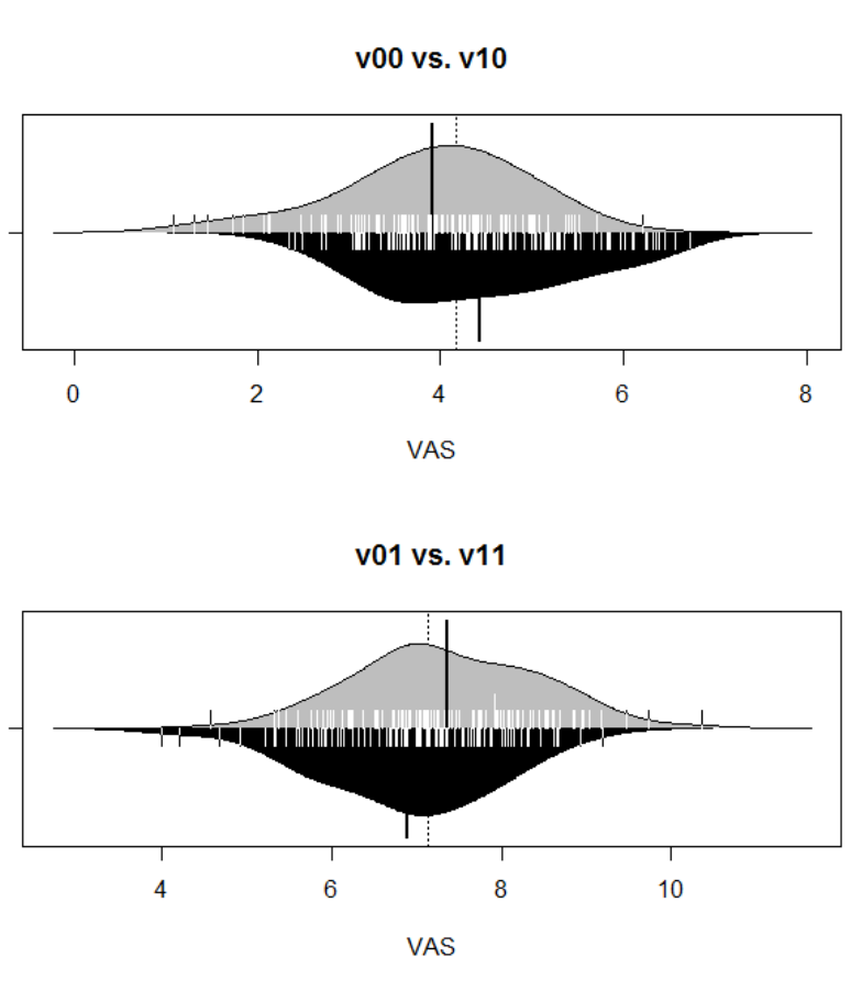
263
Figure 61. Beanplots depicting the differences in means and various distributional
characteristics of the dataset.

264
Table 30
Paired samples t-tests and nonparametric Wilcoxon signed-rank tests.
95% CI for Location
Parameter
95% CI for
Effect Size
Test
Statistic
df
p
VS-
MPR*
Location
Parameter
SE
Difference
Lower
Upper
Effect
Size
Lower
Upper
v00
-
v01
Student
3.418
99
9.169e -
4
57.360
0.520
0.152
0.218
0.822
0.342
0.139
0.543
Wilcoxon
3439.000
0.002
34.201
0.508
0.209
0.827
0.362
0.152
0.541
v10
-
v11
Student
-3.102
99
0.003
24.525
-0.470
0.152
-0.771
-0.169
-0.310
-0.510
-0.109
Wilcoxon
1688.000
0.004
16.570
-0.467
-0.774
-0.145
-0.331
-0.516
-0.118
* Vovk-Sellke Maximum p -Ratio: Based on the p -value, the maximum possible odds in favor of H over H equals 1/(-e p log( p ))
for
p ≤ .37 (Sellke, Bayarri, & Berger, 2001).
Note. For the Student t-test, location parameter is given by mean difference d ; for the Wilcoxon test, effect size is given by the
Hodges
-
Lehmann estimate.
Note. For the Student t-test, effect size is given by Cohen's d ; for the Wilcoxon test, effect size is given by the matched rank biserial
correlation.

265
5.4.2 Bayes Factor analysis
The Bayesian model we specified was isomorphic to Experiment 2, i.e., we specified
the same noncommittal “objective Bayes” Cauchy priors (cf. Gronau et al., 2017).
H
1
: δ Cauchy(0,r)
The Bayes Factor for the first comparison (experimental condition V
00
vs. V
01
) resulted
in a Bayes Factor of BF ≈ 24.05, i.e., P(D│H
1
) ≈ 24.05 and conversely P(D│H
0
) ≈
0.04. The BF for the second contrast (V
10
vs. V
11
) was BF ≈ 9.71, i.e., and its
reciprocal was P(D│H
0
) ≈ 0.10. The results (with associated errors) are depicted in
Table 14. According to Jeffreys’ interpretational schema, the two Bayes Factors provide
strong to moderate-strong evidence for H
1
. Descriptive statistics and the associated 95%
Bayesian credible intervals are given in Table 15. In addition, the results are visualised
in Figure 62. A complete summary of the results of the Bayes Factor analysis is
available under the following URL: http://irrational-decisions.com/phd-
thesis/bayesfactor-analysis-exp4.html
In addition, we uploaded the underlying JASP analysis script to facilitate analytical
reviews as suggested by Sakaluk, Williams, & Biernat (2014): http://irrational-
decisions.com/phd-thesis/analysis-script-exp4.jasp
Table 31
Bayes Factors for both orthogonal contrasts.
BF
error %
v00
-
v01
24.050
6.998e -7
v10
-
v11
9.707
1.725e -6
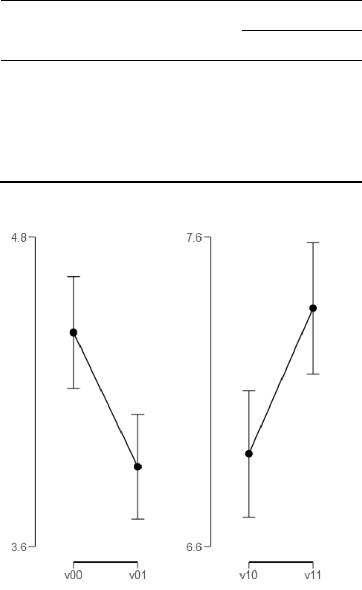
266
Table 32
Descriptive statistics with associated 95% Bayesian credible intervals.
95% Credible Interval
N
Mean
SD
SE
Lower
Upper
v00
100
4.430
1.090
0.109
4.214
4.646
v01
100
3.910
1.020
0.102
3.708
4.112
v10
100
6.900
1.030
0.103
6.696
7.104
v11
100
7.370
1.070
0.107
7.158
7.582
Figure 62. Means per condition with associated 95% Bayesian credible intervals.
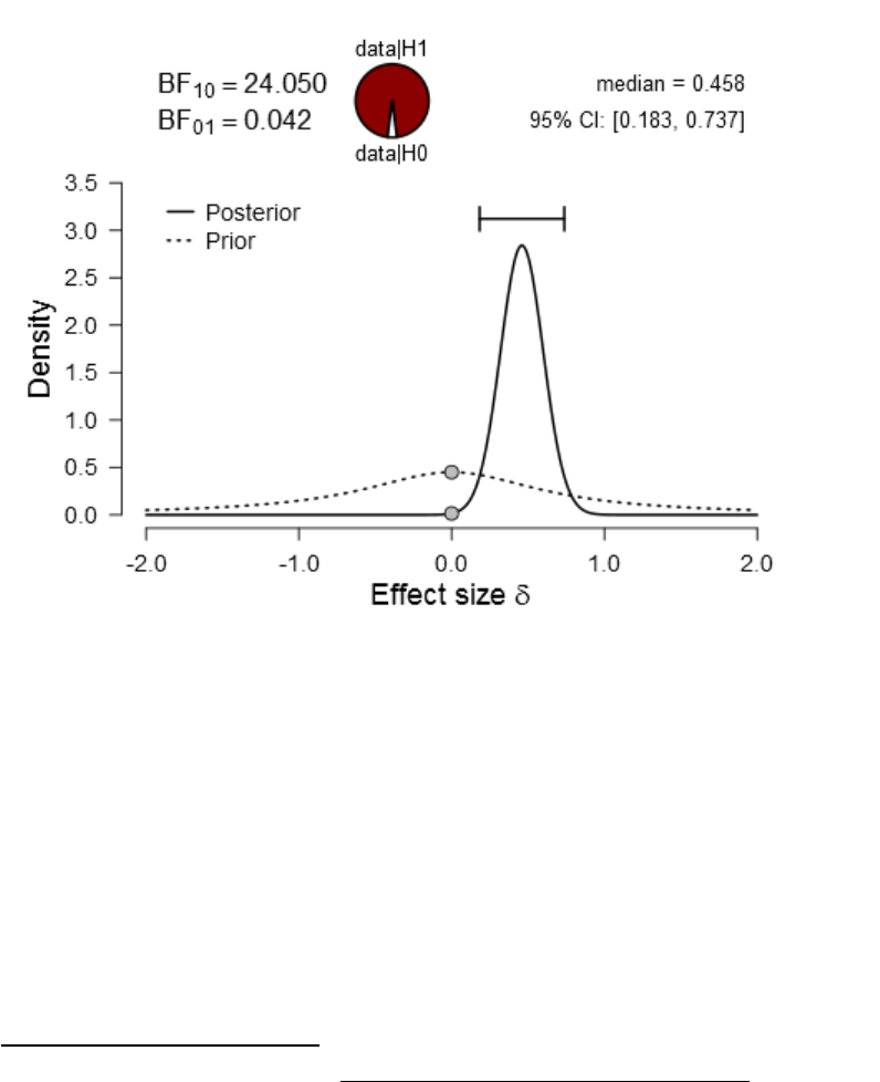
267
A visual summary of the most important analytic results is given in Figure 63 and
Figure 64. The figures are composed of: 1) a visualisation the prior distribution of the
effect sizes, 2) the associated posterior distributions, 3) the associated 95% Bayesian
credible intervals, 4) the posterior medians, 5) the Bayes Factors, 6) the associated
Savage–Dickey density ratios
149
(E. J. Wagenmakers et al., 2010), 7) pie-charts of the
Bayes Factor in favour of H
1
.
Figure 63. Prior and posterior plot for the difference between V
00
vs. V
01
.
149
For an interactive visualisation see http://irrational-decisions.com/?page_id=2328
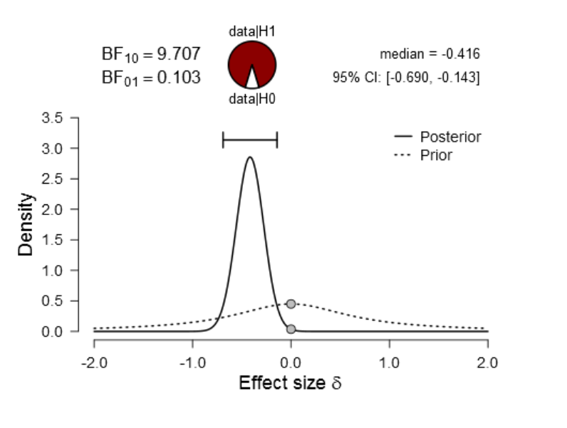
268
Figure 64. Prior and posterior plot for the difference between V
10
vs. V
11
.
As in Experiment 2, we performed Bayes Factor robustness checks for a range of
Cauchy priors per comparison. The results indicated that the evidence for H
1
was robust
under various parametrisations. For the first contrast (V
00
vs. V
01
) the maximum BF was
obtained at r ≈ 0.29 (max BF
10
≈ 32.26) and for the second contrast (V
10
vs. V
11
) at r ≈
0.26 (max BF
10
≈ 14.03). Details of the robustness check are given in Figure 65 and
Figure 66, respectively. Similar to the previous analyses, we computed a sequential
Bayes Factor analysis to investigate the accrual of evidence in favour of over time. The
results per comparison are visualised in Figure 67 and Figure 68, respectively. It is
noteworthy that for the first comparison (V
00
vs. V
01
), there was a peak around n=50,
followed by a decline of the strength of evidence. However, in the subsequent trials
evidence increased again steadily and reached its maximum value around n=95, viz.,
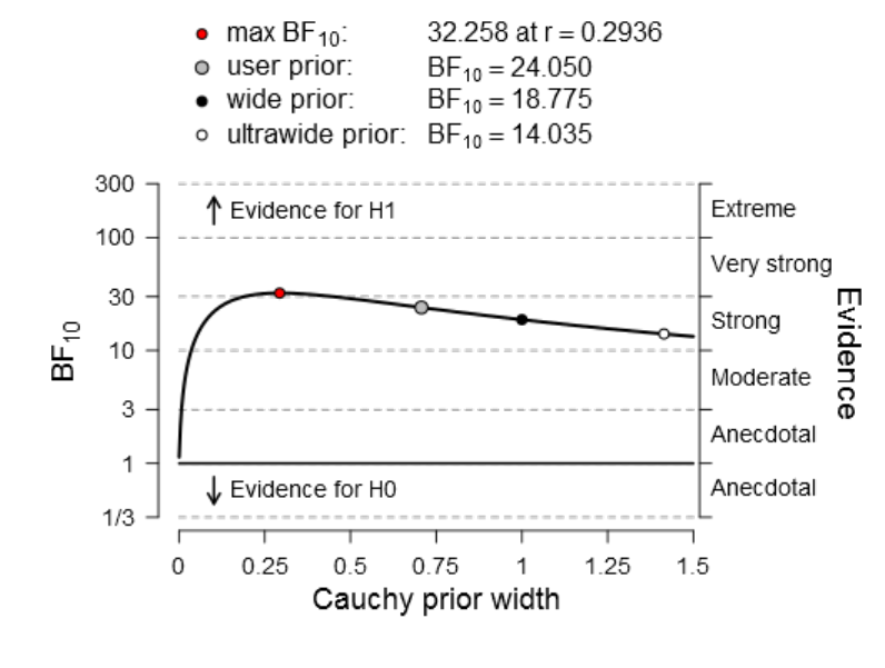
269
“strong evidence” for H
1
according to Jeffreys’ heuristic interpretational schema
(Jeffreys, 1961). For the second comparison, evidence in favour of H
1
became only
available after n=90 (ending up on the border between moderate and strong evidence for
H
1
).
Figure 65. Bayes Factor robustness check for condition V
00
vs. V
10
using various
Cauchy priors.
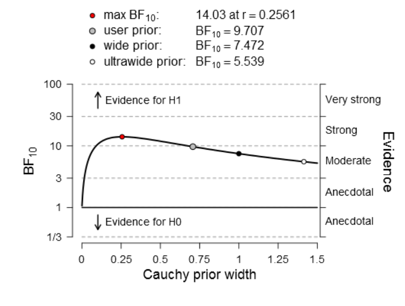
270
Figure 66. Bayes Factor robustness check for condition V
01
vs. V
11
using various
Cauchy priors.
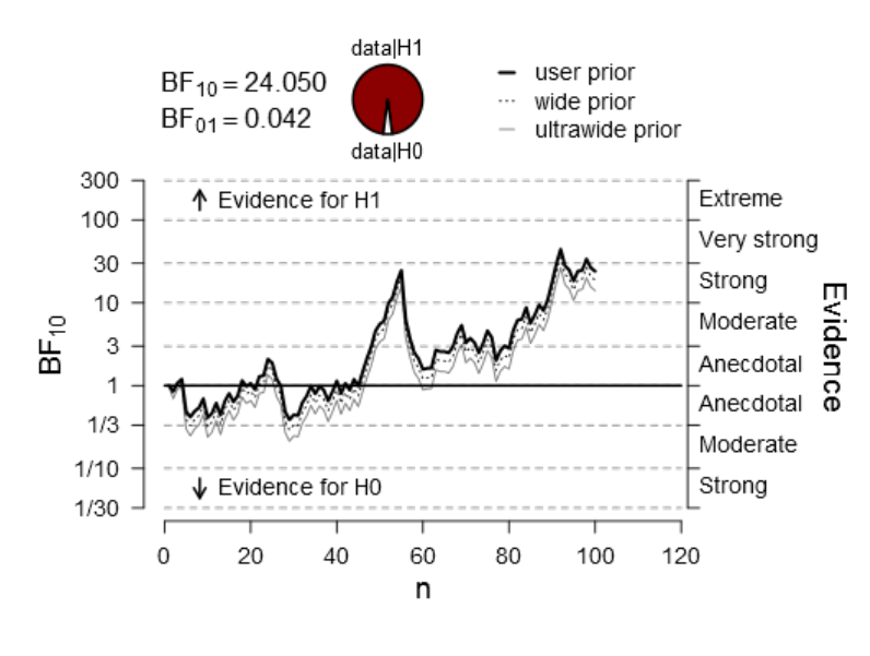
271
Figure 67. Sequential analysis depicting the accumulation of evidence as n accumulates
over time (for experimental condition V
00
vs. V
10
).
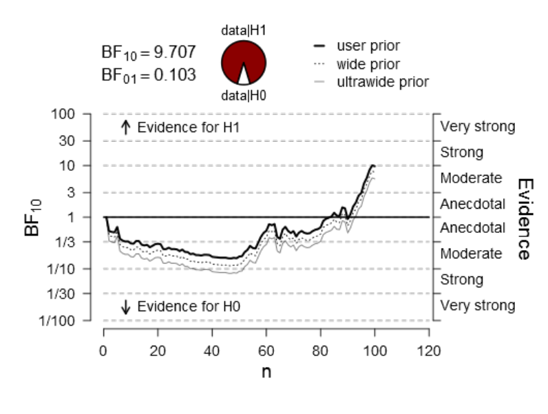
272
Figure 68. Sequential analysis depicting the accumulation of evidence as n accumulates
over time (for experimental condition V
00
vs. V
10
).
5.4.3 Bayesian a posteriori parameter estimation using
Markov chain Monte Carlo methods
This section reports the application Bayesian parameter estimation via Markov chain
Monte Carlo (MCMC) methods to the data of Experiment 4. It has been demonstrated
that MCMS methods are a very powerful approach to statistical analysis and inference
(Gelman et al., 2004). Specifically, we conducted Bayesian analyses with computations
performed by the Gibbs-sampler JAGS (Plummer, 2005). JAGS is a “flexible software
for MCMC implementation” (Depaoli et al., 2016). We were particularly interested in
measures of central tendency derived from the posterior distribution in order to evaluate
273
differences between experimental conditions. However, we also estimated additional
metrics (e.g., quantiles) of the posterior to gain a more complete picture.
5.4.3.1 Bayesian parameter estimation for the difference between
experimental condition V
00
vs. V
01
We utilised the same hierarchical Bayesian model as described in Experiment 2. That is,
we specified the same priors on all parameters and performed the simulation with the
same specifications. As in the previous analysis, we performed the MCMC simulation
with 100000 iterations, 500 adaptation steps, and 1000 burn-in steps (no thinning, 3
Markov chains in parallel). We will first report the convergence diagnostics and we will
then proceed to examine the posterior distributions.
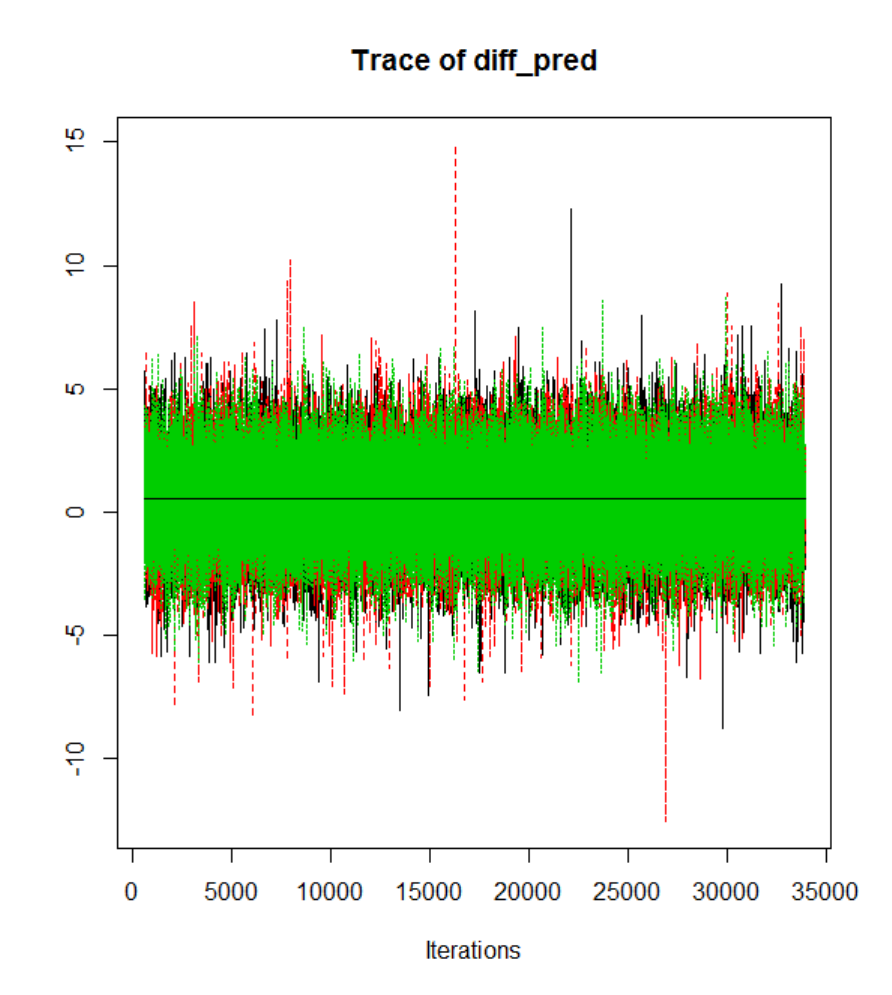
274
5.4.3.2 Markov chain Monte Carlo simulation output analysis and
convergence diagnostics
Figure 69. Trace plot of the predicted difference between means for one of the three
Markov Chains. The patterns suggest convergence to the equilibrium distribution π.
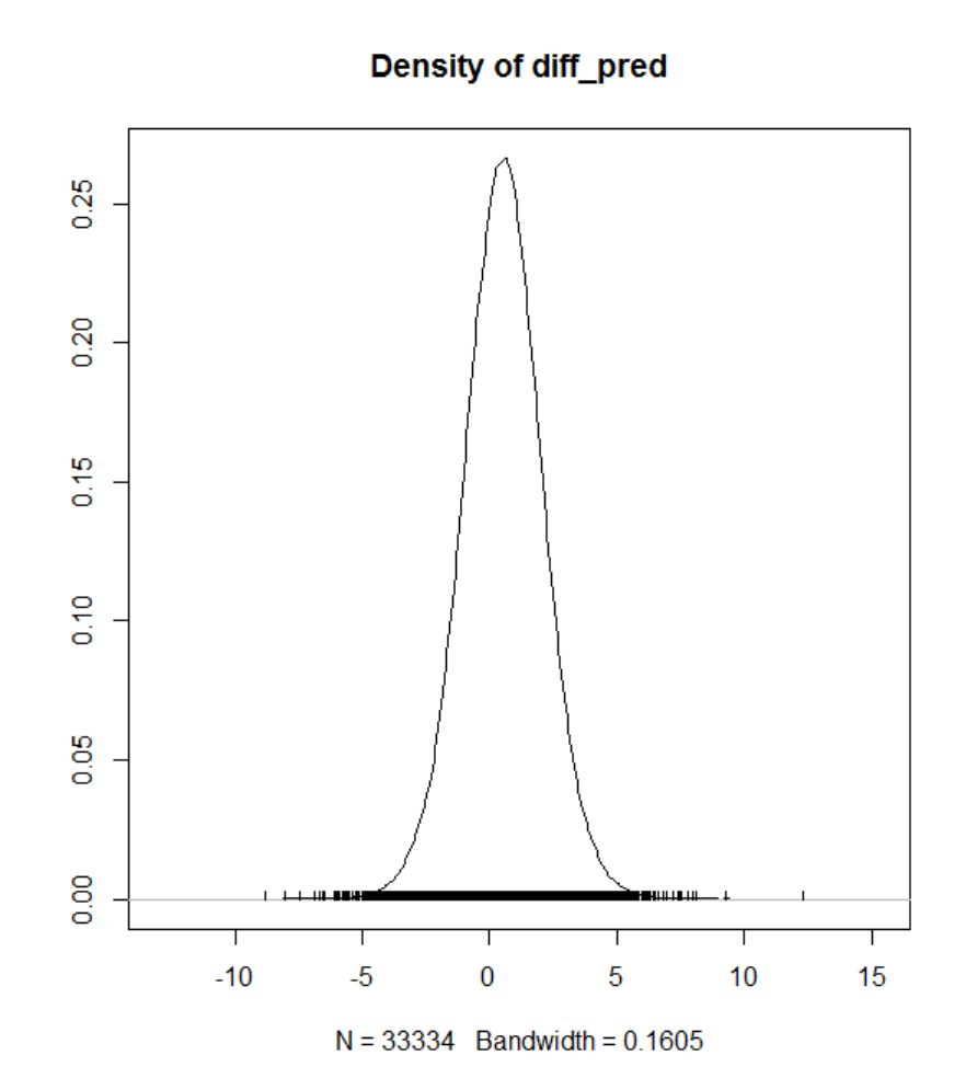
275
Figure 70. Density plot for the predicted difference between means.

276
Table 33
Summary of selected convergence diagnostics.
Iterations = 601:33934
Thinning interval = 1
Number of chains = 3
Sample size per chain = 33334
mean sd mcmc_se n_eff Rhat
mu_diff 0.524 0.182 0.001 65510 1.000
sigma_diff 1.466 0.143 0.001 45218 1.000
nu 37.497 29.840 0.214 19470 1.001
eff_size 0.361 0.129 0.001 65616 1.000
diff_pred 0.529 1.571 0.005 100633 1.000
Model parameters:
• μ
∆
(mu_diff): The estimated mean pairwise difference between experimental
conditions
• σ
∆
(sigma_diff): the scale of the pairwise difference (a consistent estimate of SD
when nu is large)
• ν (nu): The degrees-of-freedom for the bivariate t distribution fitted to the
pairwise difference
• δ (eff_size): the effect size calculated as (
0)/
.
• μ
∆pred
(diff_pred): predicted distribution for a new datapoint generated as the
pairwise difference between experimental conditions

277
Convergence diagnostics:
• mcmc_se (Monte Carlo Standard Error, MCSE): The estimated standard error of
the MCMC approximation of the mean.
• n_eff (Effective Sample Size, ESS): A crude measure of effective MCMC
sample size.
• Rhat (Shrink factor,
): the potential scale reduction factor (at convergence,
1).
Table 34
Results of Bayesian MCMC parameter estimation for experimental conditions V
00
and
V
10
with associated 95% posterior high density credible intervals.
mean median mode HDI% HDIlo HDIup compVal %>compVal
mu 0.518 0.517 0.520 95 0.215 0.826 0 99.9
sigma 1.500 1.495 1.485 95 1.280 1.730
nu 43.814 35.648 20.242 95 4.642 105.639
log10nu 1.542 1.552 1.556 95 0.961 2.112
effSz 0.347 0.346 0.346 95 0.142 0.561 0 99.9
As can be seen in Table 34, the posterior difference of means μ
∆
is ≈ 0.52 with a 95%
HDI of [0.22, 0.83]. Taken together, the results of the Bayesian parameter estimation
closely converge with the those of the Bayes Factor and frequentists analysis reported
previously.

278
Figure 71. Comprehensive summary of the Bayesian parameter estimation.
Left panel: Posterior distribution of the difference between means (experimental
condition V
00
vs. V
10
) with associated 95% high density credible intervals, and ROPE [-
0.1,0.1] the standard deviation, of the estimated difference and the corresponding effect
size. Right panel: Posterior predictive plot (n=30) for the mean difference. The
normality parameter log
10
(ν) with accompanying 95% HDI.

279
Based on the ROPE/HDI decision algorithm described before (see Experiment 1), it can
be concluded that the difference between experimental conditions is credible from a
Bayesian parameter estimation point of view.
5.4.3.3 Bayesian parameter estimation for the difference between
experimental condition V10 vs. V11
Table 35
Summary of selected convergence diagnostics.
Iterations = 601:33934
Thinning interval = 1
Number of chains = 3
Sample size per chain = 33334
mean sd mcmc_se n_eff Rhat
mu_diff -0.484 0.170 0.001 64751 1.000
sigma_diff 1.359 0.137 0.001 40827 1.000
nu 35.203 29.187 0.219 17750 1.001
eff_size -0.360 0.131 0.001 60239 1.000
diff_pred -0.482 1.468 0.005 99761 1.000
Table 36
Results of Bayesian MCMC parameter estimation for experimental conditions V
10
and
V
11
with associated 95% posterior high density credible intervals.
mean median mode HDI% HDIlo HDIup compVal %>compVal
mu -0.465 -0.466 -0.467 95 -0.768 -0.162 0 0.161
sigma 1.479 1.475 1.467 95 1.247 1.716
nu 39.423 31.058 15.418 95 3.315 98.429
log10nu 1.483 1.492 1.550 95 0.860 2.083
effSz -0.317 -0.316 -0.312 95 -0.527 -0.108 0 0.161
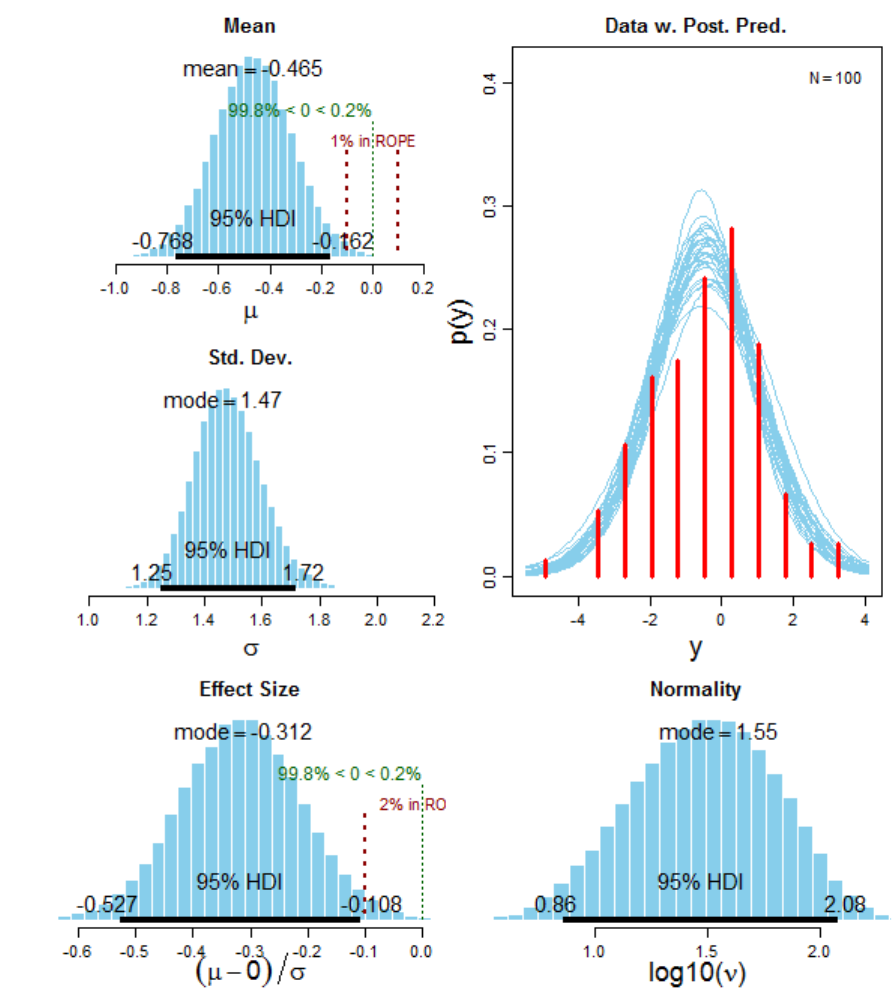
280
Figure 72. Posterior distributions for the mean pairwise difference between
experimental conditions (V
10
vs. V
11
), the standard deviation of the pairwise difference,
and the associated effect size, calculated as (
0)/
.
It can be seen in Figure 72 that the ROPE for the difference between means does not
overlap with the 95% HDI. It can thus be concluded that the difference of means in of

281
practical significance from a Bayesian parameter estimation point of view. Moreover,
the ROPE for δ did not overlap with the 95% HDI.
In sum, we concluded that the difference of means between experimental conditions V
00
vs. V
01
and V
10
vs. V
11
are credible. That is, both pairwise comparisons resulted in
values that were credibly different from zero. Hence, we rejected H
0
for both
hypotheses (i.e., μ
1
≠ μ
2
). The conclusion is motivated by the position of the
corresponding 95% equal-tail HDI for Δ
(μ1-μ2)
relative to the region of practical
equivalence. This conclusion is congruent with the inferential conclusion based on the
previous frequentists NHST and Bayes Factor analysis.
5.5 Discussion
The results of Experiment 4 were isomorphic with those obtained in Experiment 2 and
thus provided further support for the generalisability and modality-nonspecificity of our
a priori predictions. Given that the experiments were directly commensurable, the
present findings can be regarded as an empirical cross-validation and corroborate the
predictions derived from the quantum cognition model (cf. White et al., 2015, 2014b).
Moreover, our statistical analyses went beyond conventional (naïve) NHST (G
Gigerenzer, 1998, 2004; Hoekstra et al., 2014; Kruschke, 2013) by combining various
complementary mathematical/analytic frameworks (analytic triangulation). Our logical
conclusions are therefore more firmly grounded than those which rely exclusively on
orthodox (but logically invalid
150
) NHST.
150
For a discussion of the widely misunderstood syllogistic logic behind NHST see Jacob Cohen’s
excellent contributions (Cohen, 1994, 1995) and section Error! Reference source not found..
282
CHAPTER 6. GENERAL DISCUSSION
Taken together, our experimental findings lend empirical support to the predictions of
the QP model in the domain of psychophysical measurements. Specifically, the results
support the notion that cognitive processes can be modelled in terms of quantum
principles such as 1) noncommutativity of psychological observables and 2) the
constructive nature of psychophysical measurements. Furthermore, the results of our
complementary statical analyses supported our a priori predictions unequivocally
(which is not necessarily the case as NHST does not necessarily produce the same
results as Bayes Factor analysis which in turn can theoretically significantly diverge
from the inferential conclusions drawn from Markov chain Monte Carlo Bayesian
parameter estimation methods).
Specifically, the results of Experiment 1 and 3 confirmed our a priori predictions in
different sensory modalities (psychophysical noncommutativity effects in sequential
photometric versus audiometric judgments). That is, the results of Experiment 3
replicated those obtained in Experiment 1 and thereby supported the modality-
nonspecificity and generalisability of our results. The data are in line with the general
predictions formulated by Atmanspacher and colleagues (Atmanspacher, 2014, 2016;
Atmanspacher & Römer, 2012b). Moroever, the data obtained in Experiment 1 and 3
are homologous to the noncommutativity effects observed in the domain of
political/attitudinal decisions discussed in the introduction. The data thus lends to
support to the notion that noncommutativity is a fundamental feature of cognitive
operations in humans. The domain-nonspecificity of noncommutativity is a very
interesting finding and we will discuss potential fututure experiments along these lines
in § 6.12. Particularly, it would be interesting to investigate whether the effects are not
only generalisable across cognitive domains and perceptual modalities but also across
283
the phylogenetic spectrum, for instance, in other non-human life-forms, like rodents,
bacteria, fungi, et cetera. This kind of investigation would contribute to the
establishment of fundamental (unifying) principles of decision-making across diverse
domains and species. Such an interdisciplinary research program could be summarised
under the header: “The phylogeny of decision-making principles”.
In sum, the findings support the generic prediction that “non-commuting operations
must be expected to be the rule rather than the exception for operations on mental
systems” (Atmanspacher, 2014a, p. 24). This statement has far-reaching implications
for cognitive science (and many other disciplines) as commutativity is one of the
unquestioned (taken-for-granted) axioms. In other words, Kolmogorovian/Boolean
models are the de facto status quo in many scientific disciplines. Interestingly, the so
called “status quo bias” (Kahneman, Knetsch, & Thaler, 1991) describes the human
tendency to accept the status quo when faced with conflicting choice alternatives. We
suggest that this bias also applies to decision between traditional
Kolmogorovian/Boolean probability models and quantum models. That is, given the
choice many researchers might think in terms of classical probabilities and disregard
novel alternatives (cf. “loss aversion”). A cogent evolutionary/memetic argument could
be developed for this class of cognitive biases which avoid “risky exploration” of novel
territory. The need to belong and the physical danger associated with deviating from the
group/herd significantly shaped our unconscious thought processes. Today humans no
longer fear wild predators but deviating from the “memetic” group-norm is associated
with other risks in the modern world. Rejecting “the default” (e.g., the predominant
statistical model) is a difficult choice and neuroscientific imaging studies indicate that
specific prefrontal-basal ganglia dynamics are involved in overcoming the status quo
bias (S. M. Fleming, Thomas, & Dolan, 2010). However, for reasons of parsimony and
284
concision we will only adumbrate the possibility of such an evolutionary/organic
explanation which would necessarily involve a discussion of neuronal pathways
associated with nonconformity and response suppression (cf. Bari & Robbins, 2013).
An open question concerns the exact nature of the mechanisms which underpin the
cognitive mechanisms. Do the mechanisms which underlie noncommutativity take place
at the level of the retina (i.e., at the photoreceptor level) or is noncommutativity caused
by higher-order cognitive processes. In other words, where are the responsible processes
neuroanatomically located? Do they take place higher-up in the processing hierarchy of
the visual system, for example in higher-order association cortices (J. Y. Jung,
Cloutman, Binney, & Lambon Ralph, 2017)? What role do top-down influences play in
psychophysical noncommutativity? Are hierarchical neuropsychological models of
visual and auditory perception appropriate? Are introspective psychophysical
measurement effects caused by the collapse of the mental wave-function (Conte,
Khrennikov, Todarello, Federici, & Zbilut, 2009) or is some other interference process
involved? Our research cannot conclusively answer these important questions
concerning the exact mechanisms which underlie perception. However, embedded in a
broader empirical context (e.g., Z. Wang et al., 2013), our results corroborate the notion
that perception is a constructive process and that introspective measurements of
psychological observables change the cognitive variable(s) under investigation. In sensu
lato, the concept of quantum indeterminacy thus appears to be pertinent for cognitive
processes. In combination with other empirical findings (White et al., 2015, 2014b;
Yearsley & Pothos, 2014), our results challenge a fundamental assumption which forms
the basis of most cognitive models, namely that cognitive variables are always in a
determinate state which can be objectively measured (i.e., interference-free). We
propose the term “cognitive indeterminacy” as an analogon to quantum indeterminacy

285
to demarcate this aspect of the QP model from “cognitive determinism” which form the
mainly unquestioned basis of most cognitive and neuropsychological models (cf.
Popper, 1950). The term cognitive indeterminacy implies that cognitive variables are
undetermined unless they are measured. This account stands in direct contrast with
cognitive determinism which stipulates the cognitive system is always in a fixed state
which can theoretically be objectively measured without measurement-induced
perturbation. The implications of this distinction are far reaching and deserve further
systematic investigation. It has been noted before that “behavioral scientists of all kinds
are beginning to engage the issues of indeterminacy that plagued physics at the
beginning of the twentieth century” (Glimcher, 2005, p. 25) and the topic of (visual)
indeterminacy has recently connected the arts with the sciences (Pepperell, 2006, 2011).
The quantum physical concept of “counterfactual definiteness” appears thus relevant
beyond physics and particularly for psychological measurements. Counterfactual
definiteness refers to the ability to speak of the outcome of measurements that have not
yet been carried out. In the words of Asher Peres representing the traditional
Copenhagen interpretation: “unperformed experiments have no results” (A Peres, 1978).
By contrast, in the context of the many-worlds interpretation of quantum mechanics
(Everett, 2004; Tegmark, 2010; Tipler, 2000) it has been stated that "the many-worlds
interpretation is not only counterfactually indefinite, it is factually indefinite as well”
(Blaylock, 2009).
In quantum physics, the “observer effect” fundamentally changed the nature of physical
models. We argue that the same holds true for cognitive models.
151
We can no longer
151
The “Renninger negative-result experiment” is a paradoxical Gedankenexperiment posed in 1953 by
the German physicist Mauritius Renninger demonstrates one of the conceptual difficulties associated with
measurement and wave-function collapse in quantum mechanics. Renninger described a negative result
experiment as a situation in which the detector does not detect anything. The lack of detection of a
particle is still a measurement, albeit a “measurement without interaction”. Particilarly, Renninger states

286
unreflectively assume “cognitive realism”, that is, that measurements of the cognitive
system can be performed without changing the state under investigation. The
implications are far reaching, both theoretically and practically. Contextual
constructivism is incompatible with the notion that psychophysical and psychometric
measurements objectively “read out” properties of the system under investigation. This
implies a fortiori that the notion of a “detached” observer is no longer plausible. Every
measurement (be it introspective or objective, qualitative or quantitative) needs to be
regarded as an act of constructive interference. That is, the cognitive system is
necessarily disturbed by any kind of measurement. The distinction between weak and
strong measurements as used in quantum physics (Tamir & Cohen, 2013) should be
considered in the context of psychological measurements of cognitive variables,
especially in the context of psychophysics where perceptual properties can be
experimentally rigorously controlled. For example, in quantum measurements, the use
of an ancilla, (e.g., a current) to measure a given quantum system causes an interaction
between the measurement device and the quantum system. The mere act of probing the
quantum system correlates the ancilla and the system, i.e., the ancilla and the quantum
system are coupled. This is congruent with the “no free lunch theorem” (Ho & Pepyne,
2002): No information can be obtained without disturbing the system under
investigation. The main problem is that measurements degrade entanglement (e.g.,
quantum information) via decoherence. A weak measurement (weak disturbance) is
associated with a weak correlation between the system and the measurement device,
whereas a strong (more invasive) measurement leads to a stronger coupling between
systems. Weak measurement might help to circumvent the problem of decoherence (Y.
that a particle need not be directly detected by any measurement device in order for a quantum
measurement to occur (i.e., for the wave-function to collapse). Renningers argument is a refined variant
of the “Mott problem” formulated in 1929 by Sir Nevill Francis Mott and Werner Heisenberg (Mott,
1929).
287
S. Kim, Lee, Kwon, & Kim, 2012). However, in quantum physics there is currently no
universally accepted precise definition (or operationalisation) of what constitutes a weak
measurement and this lack of definition obviously complicates the transfer of the
concept into the psychological domain. Importantly, the kind of measurement might
determine whether an object behaves classical or non-classical. As Anton Zeilinger puts
it in his inaugural 2008 Newton lecture:
“The experimenter decides whether a system is classical or quantum by choosing the
apparatus, there is no objectivity … there is no border between the classical world and
the quantum world, it depends on your experiment” (Zeilinger, 2008).
Another important general question concerns what could be called “the unification
problem”. How does the software relate to the hardware? That is, how to the cognitive
processes relate to neuronal substrates within the brain (or even the enteric nervous
system)? This question is somewhat similar to the unification of chemistry and physics,
or the bridging of genetics and chemistry. In this case it concerns cognition and
neuroscience. Thus far, the question how quantum cognition relates to the brain (or
interrelated physical/somatic substrates) has not been extensively addressed. There are
some preliminary attempts, for instance, Stuart Hameroff attempts to relate quantum
cognition to his Orch-OR theory (an acronym for Orchestrated objective reduction;
delineated in Appendix A2) which he formulated in collaboration with Sir Roger
Penrose (Hameroff & Penrose, 2014b, 2014d; Penrose & Hameroff, 2011; Penrose et
al., 2011). That is, Hameroff attempts to explain quantum-like cognitive phenomena
with specific quantum-dynamics at the neuronal level of dendritic-somatic microtubules
which allow for topological dipole “qubits” (discussed in the associated section in the
introduction) which, ex hypothesi, could explain quantum computations at a neuronal
level. Specifically he proposes “quantum walks” (akin to Feynman's path integral) in

288
order to account for quantum models of cognition (Hameroff, 2013, 2014). However,
this is a speculative attempt without strong empirical support as the integration between
quantum processes at the neuronal level and higher order quantum processes in
cognition is still in its infancy stage. More empirical data is clerly needed. Nevertheless,
this integral line of research might turn out to be of great pertinence for many domains
of cognitive science, such as language, vision, logical reasoning, problem-solving, and
creativity. Moreover, this interdisciplinary approach addresses a deep scientific
question, namely, the relation between quantum-like cognitive phenomena and the
brain. In other words, how do quantum processes at the cognitive level connect to
neuronal processes. This important question thus addresses the unification of science
and how multiple “levels of explanation” can be integrated into a holistic coherent
picture which provides a more global meta-level of understanding.
6.1 Potential alternative explanatory accounts
In addition to the quantum cognition approach, there are several alternative explanatory
approaches which might be contrasted in order to account for the empirical results at
hand. A possible explanatory mechanism for the noncommutativity effects found in the
domain of photometric contrasts might be found at the neurophysiological level, e.g., at
the so called “front-end of visual phototransduction”.
152
However, we maintain that the
present finding cannot be parsimoniously explained in terms of specific signal
transduction characteristics at the level of photoreceptor cells. For instance, one might
152
Interestingly from both a visual science and physics point of view, when light interacts with the eye
the wave-particle duality resolves, that is, observation collapses the superpositional state into a
determinate eigenvalue. Einstein wrote the following on the seemingly paradoxical complementarity of
physical descriptions: “It seems as though we must use sometimes the one theory and sometimes the
other, while at times we may use either. We are faced with a new kind of difficulty. We have two
contradictory pictures of reality; separately neither of them fully explains the phenomena of light, but
together they do.” (Einstein & Infeld, 1938, p. 278)
289
propose that the refractory period of the “bleach and recycle process” of
phototransduction (Luo, Kefalov, & Yau, 2010) within the photoreceptive neurons of
the retina might be responsible for the observed effects. That is, specific biochemical
processes in opsin molecules (e.g., chromophore 11-cis retinal (P. Chen, Lee, & Fong,
2001)) might account for the observed noncommutativity effects. However, this
possibility can be logically ruled out due to the bidirectional nature of the observed
effects. That is, physiological mechanisms of transduction and adaptation cannot
account for noncommutativity effects in visual perceptual judgment. We argue that
noncommutativity is a cognitive phenomenon which is rooted in processes that are
neuroanatomically localised in higher-order association cortices and therefore
independent of signal transduction processes in the phototransduction cascade.
However, this fundamental discussion relates to the “complementarity of
psychophysics” (J. C. Baird, 1997) which conceptualises the field of psychophysics in
terms of sensory (neurophysiological) versus perceptual (cognitive) processes. We are
not in a position to answer this interesting question conclusively. However, we propose
that the observed noncommutativity effects are caused by perceptual (cognitive)
processes which cannot be reduced to cellular/molecular mechanisms (in accordance
with the previously discussed principle of cognitive completeness). However, this
falsifiable hypothesis should be investigated using modern neuroimaging techniques (if
possible in conjunction with single-unit recordings), for instance, in the striate cortex.
Such an experimental approach would potentially yield a deeper understanding of the
neurophysiological basis of the processes which underlie psychophysical
noncommutativity. The experiments at hand focused exclusively on the behavioural
level. Hence, we cannot draw firm conclusions about the underlying neuronal
mechanisms. Nevertheless, we can rule out specific theoretical accounts like receptor
290
bleaching due to the configurational pattern of the observed effects. We propose that the
visuo-spatial sketchpad (Quinn, 1988) in Baddeley’s tripartite model of working
memory (Baddeley, 1992, 2003) is a potential candidate for noncommutativity effects in
psychological observables. However, the constructive role of physical and
psychological measurements is much more complicated topic and requires a
reconceptualization of sciences most basic epistemological and ontological principles,
viz., naïve and local realism (as discussed earlier).
6.2 The Duhem–Quine Thesis: The
underdetermination of theory by data
The sceptical reader might ask the question argue wether the data can be explained in
terms of classical models. For instance, the scientific literature on perceptual contrast
effects contains a multitudinous corpus of experiments and theories and we do by no
means argue that there are no other explanatory frameworks (models/theories) which
can post festum (or “post experimentum”) account for the data at hand. In this this
section we will develop an argument based on the Duhem-Quine thesis why this is
necessarily the case. The following (selected) references were exclusively extracted
from the literature on pertinent contrast effects in visual brightness perception (B. L.
Anderson, Whitbread, & Silva, 2014; Arend, 1993; Blakeslee & McCourt, 2004;
Breitmeyer, Ziegler, & Hauske, 2007; Clay Reid & Shapley, 1988; Grossberg &
Todorovic, 1988; Kingdom, 2003; H. Neumann, 1996; Perna, Tosetti, Montanaro, &
Morrone, 2005; Peromaa & Laurinen, 2004; Prinzmetal, Long, & Leonhardt, 2008;
Purves, Williams, Nundy, & Lotto, 2004; Roe, Lu, & Hung, 2005; Schmidt et al., 2010;
Shapley & Reid, 1985; Tsal, Shalev, Zakay, & Lubow, 1994; Vladusich, Lucassen, &
Cornelissen, 2007).
291
The auditory literature on temporal perceptual context effects is presumably similarly
extensive. In the visual domain, additional theories of particular pertinence for the data
at hand are perceptual priming (e.g., B. P. Meier et al., 2007; Schmidt et al., 2010),
perceptual anchoring effects (e.g., B. L. Anderson et al., 2014) and theories concerning
temporal/sequential contrast (e.g., Eagleman, Jacobson, & Sejnowski, 2004), inter alia.
The literature on this subset of theories is likewise extensive (for a review on “a quarter
century of new ideas, captivating demonstrations and unrelenting controversy” in visual
brightness perception see (Kingdom, 2011)).
Contrast effects can be classified in terms of two orthogonal perceptual carryover
effects: contrast versus assimilation. Contrast occurs when the judgmenmt of the present
stimulus shifts in the direction opposite to the preceeding stimuli. On the other hand,
assimilation occurs when the judgment shifts in the direction of the preceding stimulus.
Similarly, perceptual priming occurs when a given stimulus is enhanced/weakend by the
match/mismatch between the preceding and anteceding stimuli. Moreover, within the
current experimental paradigm, perceptual anchoring could be described as the process
of creating (and maintaining) an association between the sensory/perceptual input and
the corresponding behavioural output (in form of the selection of an appropriate spatial
motor response – the rating). This process involves a symbolic reasoning component
because the task requires that percept is translated into a rating on the visual analoge
scale (VAS). Roughly speaking, the perceptual system has to interact with the motors
system which in turn interacts with a symbol system (which executes a specific output
on the VAS). The delineated procedure necessarily requires a form of symbol grounding
which is explainable in terms of the general embodied cognition framework, for
example, the spatial-numerical association of response codes (usually referred to as

292
SNARC effect) appears to be relevant in this response scenario.
153
According to theory,
this “perceptual anchor” between percept and response then influences subsequent
responses.
However, we would like to highlight that the three outlined theories
(contrast/assimilation, perceptual priming, and perceptual anchoring) deal exclusively
with the characteristics of cognitive/neuronal processes and not with the underlying
Kolmogorovian statistical assumption of commutativity which the present research
explicitly addresses (different levels of description). That is, along with other
researchers (e.g., Atmanspacher, 2014), we specifically argue that a relaxation of the
Kolmogorovian/Boolean commutativity axiom provides a novel perspective on data
which are only difficult to explain within classical frameworks. The quantum cognition
approach provides an overarching theoretical frame and classical frameworks can be
embedded within its circumference. In other terms, the quantum cognition approach
provides a generalised “covering law” and classical frameworks are special cases within
it. This nesting of meta-theories could be visualised as a Venn diagram (Venn, 1880),
see Figure 73.
153
The SNARC effect describes the phenomenon that people employ associations between numbers and
space. For example, a by study Dehaene, Dupoux and Mehler (1990) showed that probe numbers smaller
than a given reference number were responded to faster with the left hand than with the right hand and
vice versa. These results indicated spatial coding of numbers on mental digit line (similar to the VAS we
utilised). Relates studies indicate that associations between negative numbers and left hemiside (and
contrarywise, positive numbers and right hemiside). For example, in a study by Fischer, Warlop, Hill and
Fias (2004) participants had to select the larger number compared to a variable reference number of a pair
of numbers ranging from –9 to 9. The results showed that negative numbers were associated with left
responses and positive numbers with right responses. The mentioned results support the idea that spatial
association give access to the abstract representation of modality-independent numbers (e.g., brightness
ratings on a VAS).

293
Figure 73. Classical (commutative) probability theory as special case within the more
general overarching/unifying (noncommutative) quantum probability framework.
Note: Relative proportionalities are not representative of the actual theoretical scope
which remains elusive and should be empirically charted in the future.
We are unaware of any psychophysics experiment which directly investigated
photometric/audiometric contrasts in a homologous experimental design. Again, we do
not argue that the quantum model is the only explanatory framework which can account
for the data. However, it provides a very parsimonious account (a desideratum for every
scientific theory) as it does not postulate commutativity a priori as other models which
are based on Kolmogorovian logic do. Specifically, the vast majority of contemporary
cognitive and neuroscientific models (e.g., those utilising Boolean logic or Bayes'
theorem) are grounded on Kolmogorovian probability axioms which stipulate that
operators obey commutativity, i.e., P(A∩B)=P(B∩A). By contrast, quantum models are
not restricted by these aprioristic structural constraints and are therefore able to
Quantum probability
theory
(noncommutative)
Classical probability
theory
(commutative)

294
parsimoniously account for numerous empirical results which appear, prima facie,
irrational and paradoxical in the orthodox framework. Furthermore, more complex
models (e.g., perceptual priming (cf. Schacter & Buckner, 1998)) make additional
assumptions, i.e., they post festum add auxiliary hypotheses (Rowbottom, 2010) in order
to be able to explain comparable datasets (specifically, they consult so called “ad hoc
auxiliary hypotheses” (Grünbaum, 1976)). The quantum model does not make such a
priori assumption and consequently requires fewer parameters (“sparse
parametrisation”). That is, according to Occams’s razor
154
(known as lex parsimoniæ;
i.e., the problem-solving principle of parsimony of explanations), the more
parsimonious model should be preferred. In other words, this widely utilised principle
of reasoning is a form of an abduction heuristic (cf. Niiniluoto, 1999) which states that
simplicity should be favoured over complexity. In the subsequent section titled
“consilience of evidence” we develop an argument which emphasises the importance of
convergence of evidence from a multiplicity and diversity of (unrelated) sources (we
154
The principle is often stated in Latin which is helpful to precisely define its original meaning: “Entia
non sunt multiplicanda praeter necessitate” (transl. “Entities should not be multiplied beyond necessity”).
Another common expression of the principle is “Pluralitas non est ponenda sine necessitate” (transl.
“Plurality should not be posited without necessity”). From a memetic perspective, this quasi-economical
idea is not a new one and the same principle has been formulated before Occam, for instance, by Leipniz.
Leipniz in turn was predated by Aristotle and it would therefore perhaps be historically more accurate to
refer to the principle as “Aristotle's Razor” (as suggested by Charlesworth, 1956, in his eponymous
article). In his timeless classic “Posterior Analytics” Aristotle writes: “We may assume the superiority
ceteris paribus [other things being equal] of the demonstration which derives from fewer postulates or
hypotheses” (p.150). The “eteris paribus” assumption (i.e., other things being equal or “held constant”) is
essential for the systematic design of controlled empirical scientific experiments as independent variables
are usually held constant in order to be able to investigate the effect(s) of interest on the dependent
variable, which (in principle) allows for the establishment of logical/statistical relations between
observables (e.g., ANOVA/ANCOVA; analysis of variance/covariance). It is important to note that
confounding factors can never be completely ruled out because, unbeknownst to the experimenter, a
“tertium quid” (i.e., a third thing that is undefined but is related to two defined things) might causally
interfere and confound the empirical correlation (cf. Richard Rorty, 1986). Such an unknown intervening
factor might of course also be present in the current experimental context and this would of course
confound our interpretation which should be regarded as a provisional “inference to the best explanation”
(Ben-Menahem, 1990; G. Harman, 1992). Due to our extensive intrinsic epistemological limitation as
cognising human creatures we are in no position to make absolutist truth-claims. It is crucial to reiterate
that scientific knowledge is always provisional and should be revised in the light of new evidence. This
reiteration is particularly important given the many self-serving biases (e.g., confirmation bias, status-quo
bias, self-enhancement bias, etc. pp.) which a deep-seated in our cognitive system and which are
incompatible with a truly scientific modus operandi.

295
suggest the neologism “interdisciplinary polyangualtion”). We are convinced that
scientific progress requires perspectival multiplicity in order to approach a given
problem. Therefore, an experiment should never be evaluated in isolation but always in
a broader context of available evidence. Consquently, our results should be interpreted
on the basis of the outlined empirical background and as a conceptual cross-validation
(White et al., 2015, 2014b) which fits into a larger research agenda on quantum
cognition (Busemeyer & Bruza, 2012).
In addition, the question of whether alternative explanatory models are “better” than the
present one enters into the deep and spacious waters of philosophy of science. Model or
theory comparison is never objective and straightforward. It is not simply a matter of
objectively comparing various numerical goodness of fit indices for model selection
with each other (e.g., χ
2
, RMSEA, AIC, etc.).
It is important to note that the quasi-Darwinian scientific evaluation of model fitness
always has a strong implicit theoretical component. Specifically, the “Duhem-Quine
Thesis” (of underdetermination theory by data)
155
states that it is impossible to test a
scientific hypothesis in isolation because any empirical test stipulates of one or more
auxiliary hypotheses (i.e., additional background assumptions which are not part of the
formal model comparison). The underdetermination argument thus states that a given
piece of evidence/data is insufficient to decide which belief (a mental model or theory)
one should hold. This does of course not imply that model comparison is per se
impossible (a non sequitur). What this meta-theoretic reflection implies is that there are
always multiple (known or unknown) theories which fit the same dataset equally well so
that an objective empirical decision is an impossibility. Therefore, the phraseology
155
A “strong version” of the collaborative thesis was later reformulated by Quine in his essay “Two
Dogmas of Empiricism” (Quine, 1976). Quine’s influential concept of the “web-of-belief” is of great
pertinence in this respect (Quine & Ullian, 1978).
296
“underdetermination of theory by data”. Interpretations of experimental data should
therefore always take a broader empirical perspective into account. As stated before,
much of the impetus for the current investigation comes from research on
noncommutativity and constructive measurement effects which reported positive results
is completely different cognitive domains (White et al., 2015, 2014a, 2014b).
Consequently, we provided an interpretation within a holistic empirical context. The
quantum cognition approach has already been applied to a diverse body of decision-
scenarios, ranging from linguistic, to probabilistic, to attitudinal, to perceptual
decisions, inter alia (Blutner et al., 2013; Busemeyer & Bruza, 2012; Busemeyer,
Wang, & Shiffrin, 2012; Kvam et al., 2015). We thus refrain from interpreting our
results in isolation (a theoretical vacuum void of contextual-meaning or “empirical
Gestalt”). Of course, one can evoke numerous alternative post hoc explanations were
not part of the initial predictions, but this would be a very selective procedure and it
would be prone to implicit biases (e.g., confirmation-bias (Nickerson, 1998), hindsight-
bias (e.g. Hoffrage, Hertwig, & Gigerenzer, 2011)). We are aware that model
comparison is often depicted as an integral part of “selling one’s research” but we think
that deeper meta-theoretical reflections on the topic (and its positivistic assumptions)
are at least as important as “fashionable” numerical comparisons which create the
decision-theoretical impression of quantifiability and objectivity (Quine used the term
“dogma of empiricism”). We think that, generally speaking, these model-comparison
approaches (i.e., dichotomous either/or decisions) are oftentimes highly selective and
therefore of little value to the critical reader (if not detrimental because they create the
statistical “illusion of objectivity” (Berger & Berry, 1988)). Further, the Duhem-Quine
thesis asserts that no single scientific hypothesis is capable of making accurate
predictions. Scientific predictions usually require various auxiliary hypotheses

297
(oftentimes implicitly) which are oftentimes taken for granted and are therefore not
explicitly formulated.
156
A schematic visual representation of the Duhem-Quine Thesis
is depicted in Figure 74. According to this view, an ultimately decicive experimentum
crucis is thus epistemologically not feasible. This epistemic stance is incompatible with
decisions which dichotomise model comparison. Per contrast, it is theoretically
compatible with a Bayesian perspective on belief-updating which emphasises the
inherently graded nature of evidence and the importance of prior beliefs which are
regarded as crucial and which therefore have to be explicitly integrated in any
hypothesis testing/decision procedure.
Figure 74. The Duhem-Quine Thesis: The underdetermination of theory by data.
We argue that the commutativity axiom is a paradigmatic example of an a priori
accepted auxiliary hypothesis. In his extensive analysis of the philosophy of psychology
156
In addition, Gödel's incompleteness theorems are relevant in context.
Theory
A
•Auxiliary hypothesis X
1
•Auxiliary hypothesis X
2
•Auxiliary hypothesis X?
Theory
B
•Auxiliary hypothesis Y
1
•Auxiliary hypothesis Y
2
•Auxiliary hypothesis Y?
Theory
C
•Auxiliary hypothesis Z
1
•Auxiliary hypothesis Z
2
•Auxiliary hypothesis Z?
Empirical Data

298
Wittgenstein used the term “aspect blindness” to refer to the impossibility to “see”
certain phenomena which ubiquitous and therefore taken for granted. Commutativity
might such a “overlooked” phenomenon because the vast majority of scientific models
prima facie assume the validity of Kolmogorovian/Boolean logic (e.g., models in
computer science, neuroscience, cognitive science, artificial intelligence, psychology,
etc. pp.) The commutativity principle is implicitly assumed to be foundational and
therefore usually escapes scientific scrutiny (in the pertinent literature this is discussed
under the header “foundationalism” (Sosa, 1980)). Wittgenstein makes the following
concise remark on aspect blindness:
“Who follows a rule has formed a new concept. For a new rule is a new way of seeing
things” (Wittgenstein's Nachlass, 124:134–135)
159
In other words, a theoretical release from the aprioristic constrains of the commutativity
axiom might open up unforeseen novel vistas of scientific inequity. We hope that this
thesis makes a small contribution to this cognitive endeavour.
6.3 Experimental limitations and potential
confounding factors
In this section we will address several limitations of the experiments at hand and
various potentially confounding factors. We will specifically focus on 1) sampling bias
2) the operationalization of the term “measurement” and 3) response bias and the
depletion of executive resources (i.e., ego-depletion).
159
The computerized edition entitled “Wittgenstein's Nachlass” contains Wittgenstein's
complete philosophical writings and provides free access to the 20,000 facsimiles and
transcriptions (Savickey, 1998). URL: http://www.wittgensteinsource.org
299
6.3.1 Sampling bias
The vast majority of participants was sampled from the general student population. This kind of
“convenience sampling” (Etikan, 2016) can introduce potential confounds and compromises the
generalisability/external validity) of the conclusions which are based on this sample. This is
general problem which applies to a large segment of experimental scientific research (Bracht &
Glass, 1968; C. S. Lee, Huggins, & Therriault, 2014; Rothwell, 2005; Shadish William R.,
2002) because rodents and students are readily available for research. Therefore, external
validity is a serious concern when one draws generic conclusions the scientific literature. The
overarching questiong is: Is the sample at hand representative of the general population? This is
a statistical question and various sampling strategies have been discussed for a long time, e.g.,
random sampling, stratified sampling, clustered sampling, adaptive sampling, systematic
sampling, rational sub-grouping (e.g., Etikan, 2016; Foldvari, 1989; Imbens & Wooldridge,
2008; Sedgwick, 2014).
Given the fact that we conducted one of the experiments in India within a culturally very
different population we can put forth a cogent argument which support the generalisability of
our findings, specifically with respect to “cross-cultural validity” (e.g., Ember & Ember, 2009;
Schwartz et al., 2001; Sekuler, McLaughlin, & Yotsumoto, 2008). Nevertheless, we sampled
from a population of students which might possess certain (age-related) information processing
characteristics which are not representative of the general population. Therefore, future studies
should address this issue and investigate the reported effects within different age-cohorts and
within non-student populations. Importantly, psychological and gerontological research
indicates that perceptual mechanisms change significantly over the course of a lifetime
(Comalli, 1967; Humes, Busey, Craig, & Kewley-Port, 2013). Therefore, planned comparisons
between various age groups might be a fruitful research area avenue for the future.
300
6.3.2 Operationalization of the term “measurement”
It is crucial for every scientific experiment that all variables are clearly defined. However, the
literature contains an extensive debate concerning the question what exactly constitutes a
measurement. In quantum physics there is currently no universally accepted precise definition
(i.e., operationalisation) of the term. However, the exact definition is of utmost importance
because the operationalisation of the measurement process lies at the core of the the
interpretation of quantum mechanics. However, there is currently no consensus in the scientific
community and various definitions have been proposed (Penrose, Kuttner, Rosenblum, & Stapp,
2011; C. U. M. Smith, 2009; H. Stapp, 2007). From a psychological point of view, an
interesting candidate is consciousness itself (Hodgson, 2012; H. P. Stapp, 2004). According to
this view, a measurement always involves a conscious agent. This definition then relocates the
problem: What is consciousness? We will not get into this deep philosophical question here
even though it is crucial for the advancement of science as consciousness is the final frontier
(one of the “open problems”) and a topic of intense interest to a large number of scientists from
a variety of disciplines.
This lack of a precise operationalisation in physics obviously complicates the transfer of the
concept into the psychological domain of quantum cognition. Importantly, the “kind of
measurement” might determine whether an object behaves classical or non-classical. For
instance, it has been suggested that the decoherence problem can be circumvented by utilising
weak measurements (but see Y. S. Kim et al., 2012). Anton Zeilinger addressed this point in his
inaugural 2008 Newton lecture: “The experimenter decides whether a system is classical or
quantum by choosing the apparatus, there is no objectivity … there is no border between the
classical world and the quantum world, it depends on your experiment” (Zeilinger, 2008).
In the psychological experiments at hand, the measurement problem might even be more
intricate than in physics because we are dealing with “introspective psychophysical
measurements” which are, per definition, not objectively quantifiable. As researchers, we can
only indirectly infer the underlying cognitive processes because because we lack direct access to

301
the psychological interior of the cognisor. Therefore, future studies could employ neuroimaging
techniques (e.g., EEG, fMRI, EMG, PET, NIRS) in order to obtain more “direct” quantitative
readouts from the brain. These quantitative physical signals could then be correlated with the
more quantitative psychological self-report data. Such a complementary analysis would provide
a much broader picture of the processes under investigation. It would be particularly useful to
combine imaging techniques, e.g., simultaneous EEG and fMRI, as both provide insights into
different aspects of cognitive/neuronal processes. EEG has a high temporal resolution but a
relatively poor spatial resolution while the opposite holds true for fMRI. Therefore, a
combinatorial approach has several advantages which are discussed in greater detail by Ritter &
Villringer (2006). The resulting multimodal dataset would then allow the researcher to draw
joint inferences about the processes which undergird introspective measurements.
161
6.3.3 Response bias and the depletion of executive resources
(ego-depletion)
Another shortcoming of the experiments relates to the actual design. Participants had to make a
large number of repetitive (monotonous) perceptual judgments. The concept of ego-depletion is
thus relevant (Hagger, Wood, Stiff, & Chatzisarantis, 2010; Muraven & Baumeister, 2000). It is
a well-established fact that repeated decision-making depletes executive resources (which are
neuronantomically prefrontally located and which utilise a significant amount of glucose;
Baddeley’s model of working memory is pertinent in this respect; but see Appendix A7).
Therefore, one could argue that participants shift into an mode of responding which is
“cognitively economic”. That is, after a number of repetitive trials participants might reduce
their cognitive efforts and use a more unconscious/automatic modus operandi. In the literature
on decision-making humans are described as “cognitive misers” (de Neys, Rossi, & Houdé,
2013; K. E. Stanovich, Toplak, & West, 2010). In other word, depletion of executive resources
might lead to specific response biases which could confound the results in a systematic fashion.
161
However, one should keep in mind that neuroimaging is just another form of measurment which leads
arguably to a logical tautology.

302
Based on the available data we cannot rule out this confound and additional experiments are
needed to systematically address this open question empirically. In order to investigate this
hypothesis, one could conduct experiments with a varying number of trials.
162
Moreover, time-
series analysis (Lund, 2007) could be utilised to statistically investigate the trajectory of
perceptual judgments in a diachronic analysis (i.e., the study of change in a phenomenon over
time). However, an experimentum perfectum is impossible as every experimental
procedure comes with advantages and disadvantages. Moreover, the problem of the
“tertium quid” (an unidentified third element which confounds the experimental results
and thus their interpretation) is always lurking in the epistemological background. As
researchers we can never perfectly control all variables which might play a role in an
experiment, specifically because many influential factors might be completely unknown
to us, hence correlation ≠ causation (under all circumstances). Human creatures are
intrinsically very limited in their cognitive abilities (presumably because cognition was
shaped by evolutionary forces which selected for survival/reproduction and not for
veridical insight and propositional truths-values). Therefore, intellectual humility is
crucial for the progress of science. Only if one is aware that a system is deficient is one
able to develop the intrinsic motivation to improve it.
6.4 Quantum logic
Our results suggest that classical Kolmogorovian/Boolean logic might be inappropriate
for models of psychophysical processes. The axiomatic basis of Bayes’ theorem (which
is widely applied in psychophysics (e.g., Anastasio, Patton, & Belkacem-Boussaid,
2000)) is based on the commutativity principle. Therefore, the generalizability and
validity of Bayesian models needs to be questioned if psychophysical processes do not
162
We thank Dr. Christopher Berry for providing this useful suggestion.
303
obey the Kolmogorovian commutativity axiom (cf. Busemeyer et al., 2011b). Quantum
logic is counterintuitive and appears, prima facie, paradoxical and extremely irrational.
To use Richard Feynman’s words:
“… I think I can safely say that nobody understands quantum mechanics. So do not take
the lecture too seriously, feeling that you really have to understand in terms of some
model what I am going to describe, but just relax and enjoy it. I am going to tell you
what nature behaves like. If you will simply admit that maybe she does behave like this,
you will find her a delightful, entrancing thing. Do not keep saying to yourself, if you
can possible avoid it, "But how can it be like that?" because you will get 'down the
drain', into a blind alley from which nobody has escaped. Nobody knows how it can be
like that.” (Feynman, 1963)
However, Feynman’s protective and careful advice has been questioned because he
essentially argues that one should not try to understand, a statement which can be
regarded as anti-rationalistic (Echenique-Robba, 2013), i.e., it is always good to think
deeply about open scientific problems and the next generation of scientists should not
be discouraged to do so. Based on various quasi-Piagetian considerations (e.g., Bynum,
Thomas, & Weitz, 1972), we predict that future generations of scientists will be able to
incorporate quantum logic more easily because they will be exposed to this kind of
logic early on in their studies, whereas senior scientists have been habituated to Boolean
logic since the beginning of their education (the entire developmental trajectory was
overshadowed by this kind of logic). Hence, they have to overwrite the deeply
engrained conditioning which makes it much more difficult to adopt the new non-
Boolean logic. The adoption of a radically different logical axiomatic framework
requires neuroplasticity (G. S. Smith, 2013) and synaptoplasticity (e.g., synaptic long-
term potentiation in the hippocampi). Based on recent neuropsychological evidence and

304
theorizing (Carhart-Harris, Muthukumaraswamy, et al., 2016a; Carhart-Harris & Nutt,
2017; Tagliazucchi, Carhart-Harris, Leech, Nutt, & Chialvo, 2014), we suggest that the
5-HT system (particularly the 5-HT
2A
receptor) might play a crucial role in this context.
That is, it would be interesting to investigate if changes in the structure of logical
thought correlate with specific neurophysiological/neurochemical changes, for instance
connectivity changes set in motion by the serotonergic neurotransmitter system (cf.
Carhart-Harris et al., 2012).
Furthermore, if one agrees with the Sapir-Whorf hypothesis of linguistic relativism
(Lucy, 2015; Sapir, 1929), one could argue that mathematics and logic are a kind of
language and that this language influences (or in the strong version of the linguistic
relativism hypothesis “determines”) perception. It follows, that the logical frameworks
humans are exposed to during their education, axiomatically structure (if not determine)
their cognitions and perceptions in fundamental ways. Quantum logic has the potential
to change our perspective on reality due to its implications for local-realism (Giustina et
al., 2015; Gröblacher et al., 2007; Hensen et al., 2015). One could ask the following
question: Which Weltanschauung emerges if metaphysical theories like local-realism
and the “laws of thought” like the Aristotelian law of the excluded middle are no longer
indoctrinated from an early developmental stage?” Only time will tell... In the early
developmental stages neuroplasticity
163
is very high and the neural circuitry for thinking
and reasoning is being formatted and structured via Hebbian processes, inter alia. At the
same time synaptic pruning is taking place at a fast pace (Luiselli & Reed, 2011).
In our view, the multifactorial problem of understanding the paradoxical nature of
quantum logic is partly due to the difficulty to represent it cognitively via somatic states
163
That is the the growth of axons and dendrites and the formation and reorganization of synapses
(Cheng, Hou, & Mattson, 2010) is much more pronounced in various “critical windows” of the
developmental stages as compared to adulthood (G. S. Smith, 2013).
305
and simulations in the premotor cortex. That is, from a grounded and embodied
cognition perspective, cognition is not computation on amodal symbols in a modular
system, independent of the brain's modal systems for (e.g., vision, audition), action
(e.g., movement, proprioception), and introspection (e.g., mental states, affect)
(Barsalou, 2008). Instead, grounded/embodied cognition proposes that modal
simulations, bodily states, and situated action underlie all of cognition. Accumulating
neural evidence supports this perspective. The question thus is: What are the sensory-
motor representations associated with quantum logic (such as superposition). Human
beings do not experience superposition of objects during their normal development of
their sensory-motor system. Hence, higher-order representations of this concept cannot
be grounded in early sensory-motor experience. This lack of grounding might explain
our difficulty to “grasp” these extraordinary logical concepts. In other words, we lack
the primitive image schemata (Lakoff, 1987) in order to represent quantum logical
concepts like superposition. Bistable visual stimuli might be the closest visual metaphor
currently available to us. However, virtual reality (VR) and mixed reality (MR)
(Milgram, Takemura, Utsumi, & Kishino, 1994) in combination with haptic interfaces
(Hayward, Astley, Cruz‐Hernandez, Grant, & Robles‐De‐La‐Torre, 2004) could be
potentially useful technological tools to enlarge our sensorimotor repertoire and to
create novel percepts in order to expand our phenomenological experiences and hence
our repertoire of mental representations. We propose the neologism “artificial qualia” in
this context to refer to qualitative phenomenological experiences which have been
specifically designed for the purpose of cognitive enhancement. If the primary axiom of
embodied cognition that thought is inherently linked to sensorimotor experiences is
correct, then it follows that the systematic manipulation of specific sensorimotor

306
experiences can be utilised as a methodological tool to shape and train the intellect.
164
Aldous Huxley uses the fitting phrase “education on the nonverbal level” (Huxley,
1989) and he cites Baruch de Spinoza in this context: “Make the body capable of doing
many things. This will help you to perfect the mind and come to an intellectual love of
god”. This resonates with the ancient science of yoga which utilises various intricate
and sophisticated physical practices (Lesser, 1986) in addition to āsana (Sanskrit: )
in order to cultivate specific states of mind , viz., to reach a state of union
(nonduality/Samādhi ). In sensu lato, this nondual viewpoint also forms the basis of
the dual-aspect monism perspective on psychophysics advocated by Gustav Fechner
and modern quantum physicists like David Bohm.
From a more pragmatic/applied point of view, new models are currently being
developed in various domains which utilise quantum logic principles, despite the
difficulties to epistemologically appreciate quantum logic (Low, Yoder, & Chuang,
2014; Moreira & Wichert, 2016a; Tucci, 1997; Ying, 2010). For instance, “Quantum
Bayesianism” in which a quantum state is utilised as “a presentation of subjective
probabilities about possible results of measurements on a system” (A. Khrennikov,
2015).
6.5 The interface theory of perception
The majority of visual/perceptual scientists assume that there is a three dimensional
world “out there” which contains real objects like, for instance, tigers and spiders
(Hoffman, 2016). These naïve realist theorists assume that evolutionary pressures
164
Animal and human studies indicate that the motor system (e.g., the premotor cortex) plays a central
role in various cognitive functions (Rizzolatti, Fogassi, & Gallese, 2002). Moreover, the cortico-
cerebellar circuit appears to be of particular importance in this respect, e.g., the symbolic representation
of action (Balsters & Ramnani, 2008).

307
shaped and constrained our perception in such a way that it approximates veridicality. In
other words, perception is assumed to provide a “true” picture of reality, albeit not a
complete one (no one would argue that humans and other animals perceive reality in its
entirety (inherent sensory and perceptual constrains, selective attention, sensory gating,
various cognitive limitations, etc.). Perceptual interface theory challenges this notion
and argues cogently that natural selection did not select for veridicality but for survival.
Veridicality should not be conflated with evolutionary fitness (B. L. Anderson, 2015).
That is, our perception of reality does not represent reality in its true form (the Kantian
“Ding an sich”, i.e.,” the thing in itself” or “the thing as such”). Perception merely
provides an interface which enables humans to survive. Evolution does not select for
ontological truth-value but for pragmatic survival mechanisms.
165
Examples of such
mechanisms are ubiquitously found in nature. Biologists and psychologists have studied
so called supernormal stimuli for a long time (Lichtenstein & Sealy, 1998; Moreno,
Lobato, Merino, & Mart??nez-De La Puente, 2008; Staddon, 1975). For instance, the
ocean city Plymouth has a substantial European Herring Gull (Larus argentatus)
population and these large seabirds display a salient red dot which is located on anterior
part of their rather large beak (see Figure 75). Ornithologists report that the red dot on
the adult seagulls beak has an important evolutionary function. It provides a visual cue
for the offspring in the context of feeding behaviour. Seagull chicks are attracted by the
red dot and start pecking in its presence. This simple visual cue has thus a crucial
survival function in an evolutionary context. Nobel laureate
166
Nikolaas Tinbergen
studied social behaviour patterns in various animals (he is regarded as the founder of
ethology) and conducted insightful experiments with seagulls (Tinbergen, 1951).
165
This has been experimentally demonstrated using Monte Carlo simulations of evolutionary games and
genetic algorithms (Hoffman & Prakash, 2014).
166
URL: https://www.nobelprize.org/nobel_prizes/medicine/laureates/1973/

308
Specifically, he systematically varied the properties of the adult beak and observed the
effects on the behaviour of the offspring. He concluded that the reaction (pecking
response) to the visual cue was innate and hence genetically coded. Tinbergen created
supernormal simulacra (e.g., longer and thinner beak morphology combined with
variable dot sizes) and observed that herring gull chicks pecked more frequently at
seagull cardboard models with pronounced red dots as compared to the normal adult
herring gull beaks (ten Cate, 2009; Tinbergen & Perdeck, 1950). That is, the offspring
reacted more intense to the supernormal artificial stimuli than to the real beaks (colour
was of no significant importance, what mattered was contrast and size and the form of
the beak). In other words, the supernormal stimuli “hijacked” the innate instinctual
response pattern (“innate releasing mechanism”). Tinbergen’s student Richard Dawkins
conducted similar experiments and supernormal stimuli have been found for many
species including humans. For example, the multi-billion pornography industry uses
supernormal visual stimuli (here it is clicking rate instead of pecking rate), as do
globalised fast-food chains like McDonalds in their ubiquitous PR campaigns. The
exploitation of evolutionary anchored supernormal stimuli is a ubiquitous strategy in
advertising. Supernormal stimuli are systematically utilized in order to activate innate
response patterns which have been “programmed” by specific natural selection
pressures, i.e., the PR industry knows how “to push the right buttons”.
167
Especially the
dopaminergic pathways and the reward system (e.g. nucleus accumbens, ventral
167
It could be convincingly argued that humans are as easily misled by simulacra as seagull chicks. For
instance, many spend their money on attractive looking fast-food which stimulates the taste buds of the
gustatory system (e.g., glutamate binding to the TAS1R1+TAS1R3 heterodimer receptors for the
umami/savoury taste) instead of investing in truly nutritious food (flavour enhancers which are
systematically designed by the chemical industry are supernormal stimuli). The list of supernormal
stimuli in our environment specifically designed by the industry to exploit innate responses is long. One
can only speculate about the epigenetics effects of such manipulations. HoweverGiven that olfactory
aversion can be epigenetically imparted to the offspring (to generation F2, (Dias & Ressler, 2014)), it
seems highly likely that such targeted manipulations have significant effects on gene methylation and
transcription.
309
tegmentum) appear to be involved in the elicitation of basic biological behaviours
(Salgado & Kaplitt, 2015). However, in the context of the perceptual interface theory it
has been cogently argued that the chick’s perceptual category “food bearer” is not a
realistic representation of the true characteristics of the food-bearing parent (Hoffman,
2016). The perceptual interface of the chick does not provide a statistically accurate
approximation of the real world (as argued by Bayesian models). Perception utilises a
simplified (user friendly) interface which is based on superficial symbols that enable
survival/reproduction, nothing more and nothing less. Because this Darwinian interface
evolved over the course of millennia it has a good fitness-function in a given
environmental context. However, when experimental scientist like Tinbergen enter this
environment this useful interface can be dismantled and manipulated. It is important to
note that the interface is generally mistaken for reality (again, the Kantian “Ding an
sich”), a case of epistemological naivete. Only metacognitive processes can unveil the
interface in human beings. That is, epistemology is of utmost importance in the context

310
of analysing perception.
Figure 75. Supernormal stimuli: Seagull with a natural “normal” red dot on its beak.
The interface theory (Hoffman, 2010, 2016) thus provides a novel evolutionary
perspective on perception and challenges mainstream models of perception which are
based on “Bayesian decision theory and psychophysics” (Yuille & Bülthoff, 1996).
These models argue that perception provides a faithful depiction of real-world
properties according to specific likelihood functions, i.e., perception is based on
Bayesian estimation. That is, Bayesian models of perceptions are based on the
assumption that evolution selects for veridical perceptions of reality. It is assumed that
neural networks implement Bayesian inference to estimate “true” properties of an
objectively existing external world (Hoffman & Prakash, 2014). In John Locke’s

311
dichotomous terminology: primary qualities
168
such as size, position, and are assumed
to exist before they are perceived by an observer (R. A. Wilson, 2015). According to
computational Bayesian psychophysics, perceptual biases are assumed to be caused by
prior assumptions of the perceptual system. These priors are not necessarily generic but
can be in competition (Yuille & Bülthoff, 1996). By contrast, according to perceptual
interface theory, perception does not depict reality veridically (a naïve realist
assumption) but perception provides merely a transactional (symbolic) interface (cf. the
Vedantic notion of the veiling and projecting power of Māyā discussed earlier, e.g.,
things are not what they seem to be). According to Hoffman’s theory, perception is
comparable to a simplified GUI (graphical user interface), e.g., analogues to the desktop
of a personal computer. An icon on the monitor might be be perceived to have a specific
colour and shape and location but this does not mean that the file itself has these
qualitative properties — the underlying binary computer code has no shape and colour.
When a desktop icon is physically moved this virtual movement does not literally
correspond to physical movement of code, there is no one-to-one correspondence
between those levels description. The GUI necessarily simplifies the complexity of
reality and does not represent a true state of objectively existing reality. According to
Hoffman, Samuel Johnson’s famous rejection of Berkley’s idealism illustrates the point.
Johnson kicked a stone and thought to have refuted Berkley (an invalid logical
argument aginst idealism). Hofmann reasons that “this conventionalist objection fails
because it conflates taking icons seriously and taking them literally. [...] Johnson thus
conflated taking a stone seriously and taking it literally. [...] Perhaps the answer lies in
168
Locke divides between objective primary qualities and subjective secondary properties (qualia) which
are observer-dependent such as: color, sound, taste, and odor. The interface theory of perception (and
numerous interpretations of quantum physics) challenge this dichotomisation and it has been argued that
primary qualities are identical to secodary properties, i.e., both are observer-dependent (cf. Hacker, 1986;
Priest, 1989).
312
the evolution of our interface. There was, naturally enough, selective pressure to take
its icons seriously; those who didn’t take their tiger icons seriously came to early harm.
But were there selective pressures not to take its icons literally? Did reproductive
advantages accrue to those of our Pleistocene ancestors who happened not to conflate
the serious and the literal? Apparently not, given the widespread conflation of the two
in the modern population of H. sapiens. Hence, the very evolutionary processes that
endowed us with our interfaces might also have saddled us with the penchant to mistake
their contents for objective reality. This mistake spawned sweeping commitments to a
flat earth and a geocentric universe, and prompted the persecution of those who
disagreed. Today it spawns reconstructionist theories of perception. Flat earth and
geocentrism were difficult for H. sapiens to scrap; some unfortunates were tortured or
burned in the process. Reconstructionism will, sans the torture, prove even more
difficult to scrap; it’s not just this or that percept that must be recognized as an icon,
but rather perception itself that must be so recognized. The selection pressures on
Pleistocene hunter-gatherers clearly didn’t do the trick, but social pressures on modern
H. sapiens, arising in the conduct of science, just might. “ (Hoffman, 2016, p. 12)”
In addition to its relevance for perceptual psychology, we argue that Hoffman’s theory
is highly relevant for the classical Einstein-Tagore debate (Gosling, 2007; Home &
Robinson, 1995; Sudbery, 2016) and also more generally for an understanding of
Advaita Vedānta (discussed subsequently in section 6.9). Einstein and the Indian
polymath Ravīndranātha Ṭhākura (Tagore) debated the nature of the relationship
between mind and matter (the psychological and the physical) in a personal meeting
which took place in 1930 in Berlin. Specifically, the debate between the two Nobel

313
laureates
169
focused on nonduality, epistemology, and the fundamental ontology of
reality. The crux of this dialog is also pivotal to the Einstein-Bohr debate as the
following excerpt illustrates.
Einstein: “If nobody were in the house the table would exist all the same, but this is
already illegitimate from your point of view, because we cannot explain what it means,
that the table is there, independently of us. Our natural point of view in regard to the
existence of truth apart from humanity cannot be explained or proved, but it is a belief
which nobody can lack—not even primitive beings. We attribute to truth a superhuman
objectivity. It is indispensable for us—this reality which is independent of our existence
and our experience and our mind—though we cannot say what it means.”
Tagore: “In any case, if there be any truth absolutely unrelated to humanity, then for us
it is absolutely non-existing.”
Einstein: “Then I am more religious than you are!”
Tagore: “My religion is in the reconciliation of the superpersonal man, the universal
spirit, in my own individual being.”
Einstein reformulated his famous “I don’t believe the moon only exists when I look at
it” argument in the discussion with Tagore. For Tagore, on the other hand, reality is
dependent on the human mind. These diametrically opposed positions seem
characteristic for a detached scientist who thrives for objective, rational, and sense-
independent certainty and a poet and musician who relies on intuition and subjective
phenomenological experience (i.e., science vs. art, objective vs. subjective, realism vs.
169
Einstein received his Nobel Prize in physics and Tagore in literature. Besides its cross-cultural
relevance, the dialogue can therefore also be regarded as an interdisciplinary disussion between science
and art.

314
idealism, physical vs. psychological). However, while Einstein admits that his position
is a matter of quasi-religious faith, Tagore provides rational arguments to substantiate
his position (Sudbery, 2016). Unfortunately, Einstein died before the violation of Bell’s
theorem was proven (a historical event which shed new light on the Einstein–Podolsky–
Rosen paradox which is crucial to this controversy). However, a detailed discussion of
the theoretical nexus of the interface theory of perception and its relation to the
Einstein-Tagore debate goes beyond the scope of this thesis even though the meeting of
the representatives of Western science and the Indian tradition
170
is still highly relevant
today, despite the significant progress science made in the interim (also see Gosling,
2007; Home & Robinson, 1995; Sudbery, 2016). The discussion is particularly relevant
in the context of psychophysics, quantum physics, and contemporary consciousness
studies as it addresses the nature of the relationship between the knower and the known,
the observer and the observed, the seers and the seen, psyche and physis. The main
point is that cognitive psychology, evolutionary biology, and quantum physics suggest
that “there is reason to disbelieve in preexisting physical truths” (Hoffman & Prakash,
2014) which are observer-independent. We will continue to discuss this dualistic theme
in section 6.10. We refer the interested reader to an excellent article by Donald Hoffman
in which he expounds the interface theory of perception in greater detail (Hoffman,
2016). Furthermore, a verbatim transcript of sublime discussion between Einstein and
Tagore is available under the appended URL.
171
In addition, the insightful book by
170
Einstein was already deeply impressed by the ingenuity of Indian intellectuals. For instance, Satyendra
Nath Bose (the eponym of Bosons) and Einstein developed the foundations of „quantum statistics“ (the
succesor of Maxwell-Boltzman statistics) which are based on Bose’s combinatorial formula, i.e., Bose-
Einstein statistics (Germann, 2015a; Stone, 2013). We created a website entitled „quantum dice“ which
provides a synposis of this important chapter in the history of science:
URL: http://irrational-decisions.com/quantum_dice/
171
Verbatim transcript of the Tagore-Einstein debate:
URL: https://www.scienceandnonduality.com/wp-content/uploads/2014/09/einstein_tagore.pdf
.
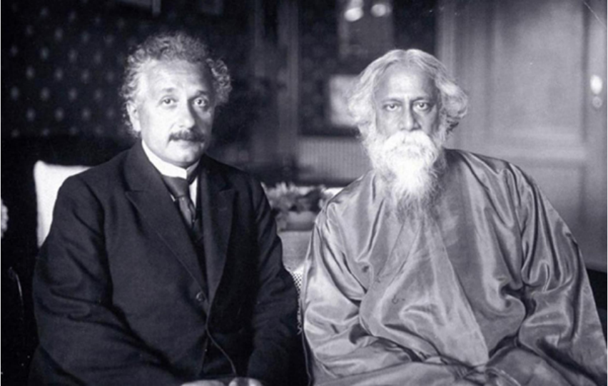
315
Gosling (2007) discusses the cross-cultural encounter and its implications for science
extensively.
Figure 76. Photograph of Albert Einstein and Ravīndranātha Ṭhākura in Berlin, 1930
(adapted from Gosling, 2007).
6.6 The Kochen-Specker theorem and the role of the
observer
The Kochen-Specker theorem (see for example Kochen & Specker, 1975) is a “no go”
theorem in physics which was mathematically proved by John Bell in 1966 and by
Simon Kochen and Ernst Specker in 1967. It conclusively demonstrates that it is
impossible that quantum mechanical observables represent objectively observable
“elements of physical reality”. More specifically, the theorem falsifies those hidden
variable theories that stipulate that elements of physical reality are independent of the
way in which they are measured (i.e. they are not independent of the measurement
316
device used to measure them and are therefore inherently contextual). That is, the
outcome of an experiment depends on how the experiment is designed and executed.
Specifically. the theorem proves mathematically that two basic assumptions of hidden
variable theories of quantum mechanics are logically inconsistent: 1) that all hidden
variables corresponding to quantum mechanical observables have definite values at any
given point in time 2) that the values of those variables are intrinsic and independent of
the device used to measure them. The inconsistency is based on the noncommutativity
of quantum mechanical observables. In colloquial language this means that the outcome
of an experiments depends crucially on how we observe things. There is no outcome
independent of the choice of measurement. That is, the features of the system we
observe do not exist a priori to measuring them (Zeilinger, 2012). As Anton Zeilinger
put it in an excellent interview: “What we perceive as reality now depends on our
earlier decision what to measure which is a very deep message about the nature of
reality and our part in the whole universe. We are not just passive observers”
(Zeilinger, 2012). This statement connects psychology and physics (which is indicative
of the deeper relevance of Gustav Fechner’s “psychophysics” discussed earlier). The
interdependence between the observer and the observed is known as the observer
problem in quantum mechanics and its pertinence for psychology has been discussed in
previous sections. In his epistemological discussions with Einstein, Niels Bohr
explicitly emphasised the role of free choice on part of the observer: “...our possibility
of handling the measuring instruments allow us only to make a choice between the
different complementary types of phenomena we want to study” (Bohr, 1996). More
recently, Rosenblum and Kuttner disagreed with Einstein when they stated that
“Quantum theory thus denies the existence of a physically real world independent of its
observations” (Rosenblum & Kuttner, 2011, p. 7). Einstein is known to have said that
317
he does not believe that the moon only exists when it is observed (Germann, 2015a;
Stone, 2013), a statement which epitomizes the widely held belief in an objectively
existing reality. However, Einstein’s ontological stance has now been conclusively
experimentally falsified (e.g., Aspelmeyer & Zeilinger, 2008; Bouwmeester et al., 1997;
Giustina et al., 2015; Gröblacher et al., 2007; Handsteiner et al., 2017). The deep and far
reaching implications of the measurement problem cannot be simply ignored. Some
physicists argue that the measurement problem is merely a “philosophical profundity”
(they use the phraseology in a derogative way) and that the problem is in reality no
problem. This is the “shut up and calculate” ethos advocated by a significant proportion
of physicists (Kaiser, 2014; Tegmark, 2007). However, as Daniel Dennett rightly
pointed out: “There is no such thing as philosophy-free science; there is only science
whose philosophical baggage is taken on board without examination.” (Dennett, 1995).
An argument which prohibits systematic thinking and the quest for understanding
should concern every scientifically minded cogniser. Replies to the advice to simply
ignore the foundational conceptual issues associated with the observer-problem have
been articulated as follows: “Shut up and let me think!” (Echenique-Robba, 2013). It
has been argued that “layers of protection against rational inquiry” have a religious
undertone. For instance, Richard Dawkins criticised religion on the following grounds:
“What worries me about religion is that it teaches people to be satisfied with not
understanding.” (Dawkins, 1996)
Contrast this with Feynman well known statement that nobody understands quantum
physics and that one should not try — otherwise bad and scary things will happen to
you!
“On the other hand, I think I can safely say that nobody understands quantum
mechanics. So do not take the lecture too seriously, feeling that you really have to
318
understand in terms of some model what I am going to describe, but just relax and enjoy
it. I am going to tell you what nature behaves like. If you will simply admit that maybe
she does behave like this, you will find her a delightful, entrancing thing. Do not keep
saying to yourself, if you can possible avoid it, "But how can it be like that?" because
you will get 'down the drain', into a blind alley from which nobody has escaped. Nobody
knows how it can be like that.” (Feynman 1964)
The blind acceptance of “that just how nature is” has been adopted by generations of
students. This has been compared to the “education” (i.e., operant conditioning) of
children who are brought up in a traditional family and who are told by their parents to
“shut up and obey” when they are still undeveloped and obedient to authority
(Echenique-Robba, 2013). The anti-rationalistic argument against deeper cogitations on
the interpretation of quantum mechanics takes many forms. For instance: “Don’t work
on this if you ever want to own a house” or “understanding is just being Newtonian” or
“whys are the unscientific business of philosophy” (but see Echenique-Robba, 2013).
We argue that psychology plays a crucial role in understanding the conceptual basis of
QM and particularly the observer-effect. Further, we propose that a deeper
understanding of consciousness (discussed in the subsequent section) and embodied
cognition will help to clean up the “conceptual mess” (Echenique-Robba, 2013) which
underpins QM. From an embodied/grounded cognition perspective, our inability to
“understand” QM (e.g., concepts like superposition) might be based on a lack of
appropriate sensorimotor representations which are usually acquired in early phases of
development (in the Piagetian stage model sensorimotor learning and development
usually takes places in a critical period which ranges from birth to about age two
(Piaget, 1952)). From this perspective, the lack of somatically anchored “primary
metaphors” (Lakoff, 1987, 1994; Lakoff & Núñez, 1998) which are required to
319
represent central QM principles is responsible for our inability to “grasp” (i.e., embody)
the conceptual basis of QM (currently QM is “ametaphorical”). According to the
grounded cognition framework, thought is fundamentally rooted in neuronal
representations associated with the perceptual and motor systems (rather than being
amodal and symbolic (Barsalou, 2008)). Therefore, the systematic development of
appropriate somatic representations might help humans to cognitively represent QM
principles in an embodied fashion, thereby enabling a genuine understanding of
seemingly paradoxical concepts via symbol grounding (cf. Gomatam, 2009). Moreover,
neurogenesis, neuroplasticity, and synaptoplasticity appear to play a pivotal role in
acquiring novel concepts. Therefore, certain neurochemical substances which facilitate
neuroplasticity and neurogenesis are important candidates in this context. For instance,
it has been shown that the nonselective 5-HT
2A
agonist psilocybin (O-phosphoryl-4-
hydroxy-N,N-dimethyltryptamine (Hofmann, Frey, Ott, Petrzilka, & Troxler, 1958;
Hofmann et al., 1959)) induces neurogenesis in the hippocampus of rats, specifically in
area CA1 (Catlow, Song, Paredes, Kirstein, & Sanchez-Ramos, 2013). The
hippocampus crucial for various forms of learning (Manns & Squire, 2001) and
learning induces long term potentiation in the hippocampus, specifically in CA1
(Whitlock, Heynen, Shuler, & Bear, 2006) which is interesting in the context of
psilocybin induced neurogenesis as these regions overlap. Moreover, functional
connectivity analysis using arterial spin labelling perfusion and blood-oxygen level-
dependent fMRI showed that psilocybin (and potentially related tryptaminergic
compounds) alters the connectivity patterns in the brain's rich-club architecture (key
connector hubs) (Carhart-Harris et al., 2012). Specifically, it facilitates more global
communication between brain regions which are normally disconnected, thereby
enabling a state of “unconstrained cognition” which might be beneficial for a deeper
320
understanding of complex problems (i.e., cognitive flexibility, divergent thinking,
creative ideation, perspectival plurality, etc.). Interestingly, synaesthesia (Hubbard,
2007; J. Ward, 2013), i.e., cross-modal associations, can be neurochemically induced in
a relatively reliable fashion. Novel cross-modal association between perceptual
modalities might be very helpful for developing new insights into the persistent
measurement problem in QM. Recall the Lockean associationism discussed in Chapter
1 in the context of synesthetic experiences: Nihil est in intellectu quod non prius fuerit
in sensu (There is nothing in the intellect/understanding that was not earlier in the
senses).
To highlight the importance of the measurement problem for science in general, the first
Newton medal awardee Anton Zeilinger explicitly states that it is not refined to the
quantum domain but it is also applicable to macro phenomena (Zeilinger, 2012).
Moreover, the problem is not only relevant for physics but particularly for psychology
and the neurosciences. From a (currently purely theoretical) material reductionist point
of view, psychology is fully reducible to its neural substrates which in turn are
composed of matter which is ultimately governed by quantum mechanical principles.
Following this hierarchical (syllogistic) argument, psychology is ultimately based on
quantum physics.
Considered from a broader perspective, the measurement problem is pertinent for the
scientific method in general because it concerns the process of objectivity of
measurements. That is, science can no longer claim detached objectivity (e.g., Pan,
Bouwmeester, Daniell, Weinfurter, & Zeilinger, 2000) because experimental findings
are significantly irreconcilable with the metaphysical and primarily taken-for-granted
assumption of local-realism (Santos, 2016) which underlies much of contemporary
scientific theorising. The measurement problem has to integrate the observer as a causal
321
force which crucially influences the outcome of measurements. That is the observer
shapes physical reality in a way which needs to be explained by physics and
psychology. As we argued previously in the context of psychophysical/introspective
measurements, we are not just passively recording but actively creating
physical/psychological observables. In this context it has been argued that physics faces
its final frontier – consciousness (H. Stapp, 2007). For instance, the “von Neumann–
Wigner interpretation”, also described as "consciousness causes collapse” of Ψ,
postulates that consciousness is an essential factor in quantum measurements. Von
Neumann uses the term “subjective perception” (J. Von Neumann, 1955) which is
closely related to the complementarity of psychophysics discussed previously. In his
seminal paper “Quantum theory and the role of mind in nature”, Henry Stapp argues:
“From the point of view of the mathematics of quantum theory it makes no sense to treat
a measuring device as intrinsically different from the collection of atomic constituents
that make it up. A device is just another part of the physical universe... Moreover, the
conscious thoughts of a human observer ought to be causally connected most directly
and immediately to what is happening in his brain, not to what is happening out at some
measuring device... Our bodies and brains thus become...parts of the quantum
mechanically described physical universe. Treating the entire physical universe in this
unified way provides a conceptually simple and logically coherent theoretical
foundation...”(H. P. Stapp, 2001). According to Stapp, two factors seem to be involved
in any measurement: the observer (the one who is asking the question) and the observed
(i.e., matter/nature). However, according to Stapp (who was a collaborator of Werner
Heisenberg), quantum theory transcendents this dualistic dichotomy between
epistemology and ontology because it was realized that the only “thing” that really
existed is knowledge. That is, ontology is always defined by epistemology which is

322
primary. In simple terms, knowledge (a faculty of the human mind) is primary and
matter secondary (i.e., Stapp argues for “the primacy of consciousness”). In a sense,
quantum physics addressed a quintessential and long-standing philosophical problem,
namely how epistemology and ontology interact and interrelate to each other. Thereby,
quantum physics overcomes this dualistic notion inherited from western philosophy
(e.g., the Cartesian split) and merges the dualistic concepts into one integrated whole.
Following this line of thought, our beliefs about reality have to be fundamentally
revised and reconceptualised. Our perspective on the relation between self and reality
will never be the same. At this point it should be emphasized that physics is still in its
infancy, even though it is one of the oldest and by far the most established science.
Notwithstanding, current physics only deals with baryonic matter
172
. Cosmologists
estimate that baryonic matter constitutes only ≈ 4% of the universe. The remaining
96% consist of dark matter and dark energy (Olive, 2010; Sahni, 2005). These numbers
show us very clearly how limited our state of knowledge with regards to the
fundamental ontology of the universe really is.
173
Psychology is a much younger than
physics and therefore “epistemological humility” is a virtue which needs to be adopted
by every scientist sincerely interested in the advancement of science and knowledge (a
“matter”
174
of scientific integrity).
172
A baryon is a composite subatomic particle made up of several elementary particles (i.e., three kinds of
quarks).
173
A fitting analogy can be drawn between our nescience concerning dark matter/energy in cosmology
and the unconscious in psychology. These limitations might be epistemological in nature. Evolution has
not equipped us humans to understand the vastness of the universe or the intricate workings of the psyche.
Our neocortical structures evolved mainly to ensure survival in our immediate environment. That is, hand
eye coordination, fight or flight responses, mating behaviour, etc. Questions concerning the nature of
reality might just be too complex for our cognitive systems. What does an ant know about computers?
With regards to consciousness a more fitting effigy might be: What does a fish know about water. That is,
there are perhaps non-negotiable epistemological limitation which deterministically delimit the human
gnostic horizon.
174
From a cognitive linguistic point of view, it is interesting to note that the English language is
extremely biased towards a materialistic worldview. Idioms and conceptual metaphors convey the

323
6.7 Consciousness and the collapse of the wave-
function
In a seminal paper, Schlosshauer (2004) summarises the foundational problems modern
physics faces. He focuses specifically on the adamantine “measurement problem” in
quantum mechanics (cf. Ballentine, 2008; Schlosshauer, 2006; Schlosshauer &
Merzbacher, 2008). This topic is to date one of the most controversial topics discussed
within science. As pointed out before, particles are assumed to exist in a superpositional
state (described by Schrödinger’s wave-equation), i.e., particles exist as mathematical
probabilistic potentialities rather than actual localisable objects. A finding which is
extensively discussed in Rosenblum and Kuttner’s book entitled “Quantum enigma:
physics encounters consciousness“ (Rosenblum & Kuttner, 2011)
175
. The key question
is how particles transform from a purely mathematical probability distribution into
actually existing objects as we observe them in everyday life? How is a quantum state
transformed into a classical state? This is the crux of the measurement problem. In the
absence of observation (measurement) particles exist in superpositional states which can
only be described in mathematical terms (interestingly the tails of the distribution are,
according to theory, infinitely long even though the probability of collapsing the wave-
function at the outer edges becomes smaller and smaller the further one moves to the
outer edges of the infinitely wide probability distribution). According to the
Copenhagen interpretation of quantum mechanics, it is the act of observation which
metaphysical ideology. For instance, the diction “it does not matter” implicitly implies that only material
things are of importance. Other languages lack this specific bias (e.g., German, Dutch, Spanish).
Conceptual metaphor theory is a powerful theoretical framework for the investigation of these linguistic
biases which structure cognition and perception (cf. Sapir-Whorf hypothesis of linguistic relativism).
According to theory, language provides a window into the underlying neuronal (sensorimotor)
representations of conceptual thought. However, given that language can be classified as a System 1
process in the dual-system framework discussed earlier (at least primarily), its effects escape our
conscious (extremely limited) awareness.
175
For a critical review see (Nauenberg, 2007) and for a response (Kuttner, 2008).
324
collapses the presumably nonmaterial and undetermined wave-function into a
determinate eigenstate /through the process of eigenselection discussed earlier).
However, no exact operational definition of what defines an “observer” and an
“observation” is provided within this theoretical framework. As Henry Stapp points out:
“… there is a sudden jump to a ‘reduced’ state which represent the new state of
knowledge” (Stapp, 1999, p.17). This “sudden jump” is a process which requires
systematic scientific investigation as it concerns the interface between psychology and
physics (i.e., the perennial question concerning the relationship between mind and
matter). The pivotal question science struggles with is: How exactly do merely
stochastic potentialities actualise? That is, how does localisable matter emerge from a
purely mathematical stochastic function (Dürr, 2001)? Stapp argues that “A superficial
understanding of quantum theory might easily lead one to conclude that the entire
dynamics is controlled by just the combination of the local-deterministic Schrödinger
equation and the elements of quantum randomness. If that were true then our conscious
experiences would again become epiphenomenal side-shows. To see beyond this
superficial appearance, one must look more closely at the two roles of the observer in
quantum theory.” (p.17)
Thus the missing piece in this quantum theory is a precise understanding of the
mechanism responsible for the collapse of the wave-function. Schlosshauser argues that
“…without supplying an additional physical process (say, some collapse mechanism) or
giving a suitable interpretation of such a superposition, it is not clear how to account,
given the final composite state, for the definite pointer positions that are perceived as
the result of an actual measurement— i.e., why do we seem to perceive the pointer to be
in one position |a
n
> but not in a superposition of positions? This is the problem of
definite outcomes.” (p.4).
325
Hence, the open question can be reformulated as follows: “Why do we not observe
superpositional states and how does the collapse which occurs because of a
measurement actually occur? One way to collapse Ψ is through an interaction with other
particles which have already taken on definite states, i.e., environmentally-induced
decoherence (Anglin, Paz, & Zurek, 1997). It is possible to measure a particle with a
measurement device and thereby collapse it via this interaction (collapse through
interaction). To be more precise, the interaction disturbs the superpositional state of the
particle. This is the decoherence effect in quantum physics and some physicist’s
hypothesis that this interaction is sufficient to account for the collapse of Ψ and the
measurement problem is thereby solved. However, in line with Henry Stapp, we argue
that this theoretical account does not really solve the problem because it leads to an
infinite regress (interestingly, this is the same problem Aristoteles described in his
classic “Posterior Analytics” when he was pondering causality. Aristotle concluded that
there must be an “unmoved mover” or a “final cause”, i.e., something that can cause
movement but does not need to be moved by itself by another external force (viz., an
“acausal causer”). In simple terms, what caused the quantum state of the particle that
causes the collapse of Ψ to collapse? This chain of causal events can be continued ad
infinitum and is therefore no real solution to the measurement problem. As Niels Bohr
already pointed out, we cannot specify the wave-function of an observed particle
separately from the other particle which is used to measure it. To paraphrase Bohr, the
wave function of the measuring particle (e.g., the measurement device) and the particle
to be measure cannot be disentangled, etc. pp., ad infinitum. The measuring particle
inherits part of the wave-function of the particle under investigation and they become
inseparably intertwined (entangled). Consequently, the particle which is measuring
cannot be explained fully without taking into account what it is measuring. One needs to

326
introduce a third particle in order to measure the measuring particle itself and the whole
process repeats itself endlessly. That is, the third particle becomes entangled with the
second and therefore the first particle. This logic leads to the infinite regression which
lies at the core of the measurement problem. This chain of measuring particles in
superposition states is called the “von Neumann chain”. From a logical point of view,
there must be something which is nonlocal and outside the entire material system (cf.
the Cartesian res cogitans vs. res extensa)
176
which escapes the regressus ad infinitum,
that is, the causal chain of events – or in Aristotelian terms “the final cause” (τέλος -
teleos). Without such finality, efficient causality becomes tautological. This
“something” (which is actually not a thing) does not obey the same physical/material
laws and it is able to cause collapse within every position within the von Neumann
chain. One candidate which has been proposed by several eminent physicists is human
consciousness (Hagelin & Hagelin, 1981; Hodgson, 2012; Penrose et al., 2011;
Rosenblum & Kuttner, 2011; H. Stapp, 2007). Taken together, this argument shows that
decoherence theory which states that interaction with the environment is sufficient to
solve the measurement problem is is incomplete. One needs to introduce another
explanatory factor into the equation order to escape the problem of infinite regress (i.e.,
circular causation).
For instance, Joos (1999) states the following: “Does decoherence solve the
measurement problem? Clearly not. What decoherence tells us, is that certain objects
appear classical when they are observed. But what is an observation? At some point we
176
Interactionist dualism (a form of substance dualism) postulates that mind and matter (psyche and
physis) are two independent and inherently different substances that can bidirectionally effect each other
in a causal manner (John R. Searle, 2007). It has been argued that the implicated phenomenon of “mental
causation” (Esfeld, 2005, 2007) is incompatible with the physical law of conservation of energy (H.
Robinson, 2016). However, others (inter alia Karl Popper, John Eccles, and Henry Stapp) argue that
interactionism is compatible with physical law if one assumes that the mental affects the physical at the
quantum (i.e., at the level of quantum indeterminacy) and that this kind of interaction might also take
place at the macroscopic level (Popper & Eccles, 1977).
327
still have to apply the usual probability rules of quantum theory.”
In the same vein Schlosshauer (2004) argues: “let us emphasize that decoherence arises
from a direct application of the quantum mechanical formalism to a description of the
interaction of a physical system with its environment. By itself, decoherence is therefore
neither an interpretation nor a modification of quantum mechanics.” (p.8)
The main problem is thus that the environment is subject to the same quantum laws and
therefore faces the same associated problems specified above. The “final” collapse
needs to be initiated by something beyond the physical system in question.
Stephen Barr (2003) describes this situation in the following terms: “The observer is not
totally describable by physics… If we could describe by the mathematics of quantum
theory everything that happened in a measurement from beginning to end-that is, even
up to the point where a definite outcome was obtained by the observer- then the
mathematics would have to tell us what that definite outcome was. But this cannot be,
for the mathematics of quantum theory will generally yield only probabilities. The
actual definite result of the observation cannot emerge from the quantum calculation.
And that says that something about the process of observation- and something about the
observer- eludes the physical description.”
The question then becomes what differentiates the observer from the physical system
under investigation. One defining characteristic is that the observer can choose between
possibilities. This is known as a Heisenbergian cut, i.e., the interface between observer
and observed. Everything below the Heisenbergian cut is describable by Ψ, whereas
everything above is described in classical deterministic terms.
A nonconscious measuring instrument cannot achieve the collapse of Ψ. According to
Henry Stapp:
328
“The observer in quantum theory does more than just read the recordings. He also
chooses which question will be put to Nature: which aspect of nature his inquiry will
probe. I call this important function of the observer ‘The Heisenberg Choice’, to
contrast it with the ‘Dirac Choice’, which is the random choice on the part of Nature
that Dirac emphasized.”
In a discussion with Einstein Bohr stated the following:
“To my mind, there is no other alternative than to admit that, in this field of experience,
we are dealing with individual phenomena and that our possibilities of handling the
measuring instruments allow us only to make a choice between the different
complementary types of phenomena we want to study.” (as cited in H. P. Stapp, 2004, p.
66)
The observer must first decide which aspect of a given system he intends to measure
and then design a measuring apparatus in order to achieve this a priori specified goal.
“In quantum theory it is the observer who both poses the question, and recognizes the
answer. Without some way of specifying what the question is, the quantum rules will
not work: the quantum process grinds to a halt.” (H. P. Stapp, 1993, p. 21)
This means that only the observer has the possibility to choose between possibilities.
Davis and Gribbin argue along the same line in their book “The matter myth” that “the
observer plays a key role in deciding the outcome of the quantum measurements – the
answers, depend in part on the questions asked.” (Davies & Gribbin, 2007, p. 307)
Summa summarum, it makes no sense to deny that the observer does not play an
essential role in the collapse of Schrödingers wave-function.
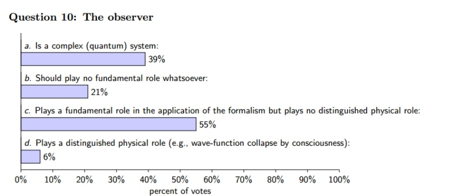
329
A recently conducted poll amonst physicist shows that the majority (55% of the sample)
admits that “the observer plays a fundamental role in the application of the formalism
but plays no distinguishing physical role”. Paradoxically, only 6% of the sample under
investigation would agree that the observer “plays a distinguished physical role (e.g.,
wave-function collapse by consciousness”). This should create cognitive dissonance
because the accept that the mathematics tells them that the observer plays a fundamental
role but they do not accept the philosophical implications which can be deductively
derived from the former statement (interestingly this is exactly the epistemological
problem Einstein faced). From a purely logical point of view this makes obviously no
sense at all. As Henry Stapp pointed out in his paper “Quantum theory and the role of
mind in nature”, this is a “metaphysical prejudice that arose from a theory known to be
fundamentally wrong”.
Figure 77. The attitudes of physicists concerning foundational issues of quantum
mechanics (adapted from Schlosshauer, Kofler, & Zeilinger, 2013; cf. Sivasundaram &
Nielsen, 2016).
In other words, even physicist who should know better implicitly (and oftentimes
explicitly) hold on to unjustifiable metaphysical beliefs that quantum mechanics
330
challenges (even in the light of clearly contradicting evidence). The superannuated
materialistic Newtonian paradigm is apparently still deeply embedded in the “modi of
thought” of the majority of western scientists (from a Kuhnian perspective this is not
particularly surprising.
This brings the discussion back in full circle to Fechner’s research agenda discussed in
the introduction. How do the psyche and physis (the inner and the outer) relate to each
other? Moreover, the emphasis on consciousness puts psychology at the centre of
modern quantum physics. It is psychology (not physics) which has systematically
studied consciousness. As science progresses, the boundaries between academic
disciplines dissolve. A hitherto unanswered question concerns the perturbation of
consciousness. If consciousness is involved in the collapse of Ψ, then systematic
alterations of consciousness might affect the collapse. The open question is: What
happens if consciousness is systematically altered?
If the collapse of the wave-function
depends on consciousness then it should be sensitive to alterations of consciousness.
Using methods of modern physics and neuropsychopharmacology, this research
question can be tested experimentally. Specifically, the 5-hydroxytryptmain (5-HT)
system seems to be of significant importance due to its central role in perceptual
processes and consciousness. The perceptual plasticity which is associated with 5-HT
2A
agonism (Carhart-Harris & Nutt, 2017) is particularly interesting in this regard.
Presently, systematic scientific research on naturally occurring mind-altering substances
(which are endogenous to human neurochemistry) is extremely limited (even though we
are currently witnessing a “psychedelic renaissance” (Bolstridge, 2013)). That is,
science is systematically neglecting a specific aspect of nature. Any model which
incorporates only a specific (selected) subset of the available quantitative and
qualitative data is necessarily at best incomplete (and in the worst-case scenario
331
prejudiced, dogmatic, and systematically biased). This is of pertinence for the thesis at
hand because complementarity of mind and matter can only be explored if both aspects
can be scientifically manipulated. Currently, matter can be manipulated (e.g., in large
hadron colliders) but manipulating certain neurochemical underpinning of cognitive
processes is still a taboo which is associated with a strong stigma (mainly propagated by
the irrational “war on drugs” initiated under Nixon (E. Wood, Werb, Marshall,
Montaner, & Kerr, 2009). Legal scholars have interpreted this situation as an attack on
“cognitive liberty” (Boire, 2000; Walsh, 2016). The recently ratified UK “psychoactive
substances act” which generically prohibits all mind-altering substances (besides the
most harmful ones (Nutt, King, & Phillips, 2010)) makes the situation even worse.
William James articulated in his classic “Essays in Radical Empiricism”:
"To be radical, an empiricist must neither admit into his constructions any element that
is not directly experienced, nor exclude from them any element that is directly
experienced"
(James, 1912/1976, p.42).
However, knowledge about the knower might be in principle impossible. The question
is: Can the experiencer be systematically investigated? In other words, can the observer
be observed? Can consciousness investigate itself? We argue that psychedelics play an
important role in this meta-cognitive (self-reflective) scientific endeavor which might
turn out to be of importance for a deeper understanding of quantum physics, given the
importance quantum physics places on observation and measurement (i.e., a truly
psycho-physical approach in the Fechnerian sense).
As Jagadguru Śaṅkarācārya pointed out in the 8
th
century AD in his commentary on the
Bṛhadāraṇyakopaniṣat 2.4.14 (one of the most ancient Upanishadic scriptures of
Hinduism (Olivelle, 1998)):
332
Even in the state of ignorance, when one sees something, through what instrument
should one know That owing to which all this is known? For that instrument of
knowledge itself falls under the category of objects. The knower may desire to know not
about itself, but about objects. As fire does not burn itself, so the self does not know
itself, and the knower can have no knowledge of a thing that is not its object. Therefore
through what instrument should one know the knower owing to which this universe is
known, and who else should know it? And when to the knower of Brahman who has
discriminated the Real from the unreal there remains only the subject, absolute and one
without a second, through what instrument, O Maitreyī, should one know that Knower?
6.8 An embodied cognition perspective on quantum
logic
“The words of language, as they are written or spoken, do not seem to play any role in
my mechanism of thought. The psychical entities which seem to serve as elements in
thought are certain signs and more or less clear images which can be “voluntarily”
reproduced and combined. […] The above mentioned elements are, in my case, of
visual and some of muscular type.” (Einstein quoted in Hadamard, 1996, The
mathematician's mind: The psychology of invention in the mathematical field.
Princeton, NJ: Princeton University Press (original work published 1945), as cited in
Diezmann, C. M., & Watters, J. J. (2000). Identifying and supporting spatial
intelligence in young children. Contemporary Issues in Early Childhood. 1(3), 299-
313).
How do people think about things they cannot see, hear, touch, smell or taste? The
ability to think and communicate about abstract domains such as emotion, morality, or
mathematics is presumably uniquely human, and one of the hallmarks of human
333
sophistication. Hitherto, the question how people represent these abstract domains
mentally has not been answered definitely. Earlier classical cognitive models act on the
Cartesian assumption of the disembodiment of mind (or soul, in Descartes terms). These
models assume that neurological events can explain thought and related notions to the
full extent. This view conforms to the computer metaphor of the mind in which thinking
is solely based on brain activity or, in computer terminology, based on the central
processing unit, also more commonly known as CPU (Seitz, 2000).
When the body is put back into thought (embodied cognition) a very different
perspective on human thinking emerges, namely, that we are not simply inhabitants of
our body; we literally use it to think. Perhaps sensory and motor representations that
develop from physical interactions with the external world (i.c., vertical dimensions) are
recycled to assist our thinking about abstract phenomena. This hypothesis evolved, in
part, by patterns observed in language. In order to communicate about abstract things,
people often utilize metaphors from more concrete perceptual domains. For example,
people experiencing positive affect are said to be feeling “up” whereas people
experiencing negative affect are said to be feeling “down”. Cognitive linguists studying
cognitive semantics (e.g., Gibbs, 1992; Glucksberg, 2001) have argued such
articulations reveal that people conceptualize abstract concepts like affect
metaphorically, in terms of physical reality (i.c., verticality). It has been argued that
without such links, abstract concepts would lack common ground and would be difficult
to convey to other people (Meier & Robinson, 2004). This approach helped scholars to
draw significant links between embodied experience, abstract concepts, and conceptual
metaphors.
Conceptual Metaphor Theory (Lakoff & Johnson, 1980) defines two basic roles for
conceptual domains posited in conceptual metaphors: the source domain (the conceptual
334
domain from which metaphorical expressions are drawn) and the target domain (the
conceptual domain to be understood). Conceptual metaphors usually refer to an abstract
concept as target and make use of concrete physical entities as their source. For
example, morality is an abstract concept and when people discuss morality they recruit
metaphors that tap vertical space (a concrete physical concept). In colloquial language a
person who is moral is described as ‘‘high minded’’, whereas an immoral person might
be denominated as ‘‘down and dirty’’ (Lakoff & Johnson, 1999). Following theory the
human tendency for categorization is structured by imagistic, metaphoric, and
schematizing abilities that are themselves embedded in the biological motor and
perceptual infrastructure (Jackson, 1983). Supporters of this view suggest that
cognition, rather than being amodal, is by nature linked to sensation and perception and
consequently inherently cross-modal (e.g., Niedenthal, Barsalou, Winkielman &
Krauth-Gruber, 2005). Furthermore, those researchers argue for the bodily basis of
thought and its continuity beyond the infantile sensorimotor stage (e.g., Seitz, 2000).
Indeed, some researchers suggest that the neurological processes that make abstract
thought possible are intimately connected with the neurological processes that are
responsible for representing perceptual experiences. Specifically, they argue that
conceptual thought is based on sensory experience, but sensory experience is not based
on conceptual thought (e.g., love is a rose, but a rose is a rose) (Meier & Robinson,
2005).
Why is an abstract concept like affect so frequently linked to concrete qualities like
vertical position? One possible explanation for this perceptual-conceptual connection
comes from developmental research. Early theorists of sensorimotor learning and
development emphasized the importance of movement in cognitive development (e.g.,
Piaget, 1952). According to this perspective, human cognition develops through
335
sensorimotor experiences. Young children in the sensorimotor stage (from birth to about
age two) think and reason about things that they can see, hear, touch, smell or taste.
Motor skills emerge and the infant cultivates the coordination of tactile and visual
information. Later researchers postulated that thinking is an extended form of those
skilled behaviours and that it is based on these earlier modes of adaptation to the
physical environment (Bartlett, 1958). For example, it has been suggested that gesture
and speech form parallel systems (McNeill, 1992) and that the body is central to
mathematical comprehension (Lakoff & Nunez, 1997).
When children get older they develop the skills to think in abstract terms. These skills
maybe built upon earlier sensorimotor representations. For example, a warm bath leads
to a pleasant sensory experience and positive affect. In adulthood, this pairing of
sensory and abstract representations may give rise to a physical metaphor (e.g., a warm
person is a pleasant person) that continues to exert effects on representation and
evaluation (Meier & Robinson, 2004). Transferred to the vertical representation of
affect one can only speculate. Tolaas (1991) proposes that infants spend much of their
time lying on their back. Rewarding stimuli like food and affection arrive from a high
vertical position. The caregiver frequently appears in the infant’s upper visual-spatial
environment (Meier, Sellbom & Wygant, 2007). As children age, they use this
sensorimotor foundation to develop abstract thought, as recognized by developmental
psychologists (e.g., Piaget & Inhelder, 1969). This early conditioning leads adults to use
the vertical dimension when expressing and representing affect. These considerations
suggest that the link between affect and vertical position may develop early in the
sensorimotor stage (see Gibbs, 2006; for sophisticated considerations).
From theory to experimental applications
336
Affective metaphors and related associations apply to a multitude of perceptual
dimensions such as, for example, spatial location, brightness and tone pitch. A plethora
of studies investigated the link between abstract concepts (i.c., affect) and physical
representation (i.c., verticality). For example, in a study by Meier and Robinson (2004)
participants had to evaluate positive and negative words either above or below a central
cue. Evaluations of negative words were faster when words were in the down rather
than the up position, whereas evaluations of positive words were faster when words
were in the up rather than the down position. In a second study, using a sequential
priming paradigm, they showed that evaluations activate spatial attention. Positive word
evaluations reduced reaction times for stimuli presented in higher areas of visual space,
whereas negative word evaluations reduced reaction times for stimuli presented in lower
areas of visual space. A third study revealed that spatial positions do not activate
evaluations (e.g., “down” does not activate ‘‘bad’’). Their studies give credit to the
assumption that affect has a physical basis.
Moreover, an often cited study by Wapner, Werner, and Krus (1957)examined the
effects of success and failure on verticality related judgements. They found that positive
mood states, compared to negative mood states, were associated with line bisections
that were higher within vertical space.
In a recent study Meier, Hauser, Robinson, Friesen and Schjeldahl (2007)reported that
people have implicit associations between God-Devil and up-down. Their experiments
showed that people encode God-related concepts faster if presented in a high (vs. low)
vertical position. Moreover, they found that people estimated strangers as more likely to
believe in God when their images appeared in a high versus low vertical position.
Another study by Meier and Robinson (2006) correlated individual differences in
emotional experience (neuroticism and depression) with reaction times with regard to
337
high (vs. low) spatial probes. The higher the neuroticism or depression of participants,
the faster they responded to lower (in contrast to higher) spatial probes. Their results
indicate that negative affect influences covert attention in a direction that favours lower
regions of visual space. In second experiment the researchers differentiated between
neuroticism and depression. They argued that neuroticism is more trait-like in nature
than depression (which is more state-like). The researchers concluded from their
analysis that depressive symptoms were a stronger predictor of metaphor consistent
vertical selective attention than neuroticism.
Similar results emerged when dominance-submission was assessed as an individual
difference variable and a covert spatial attention tasks was used to assess biases in
vertical selective attention (Robinson, Zabelina, Ode & Moeller, in press). Linking
higher levels of dominance to higher levels of perceptual verticality they found that
dominant individuals were faster to respond to higher spatial stimuli, whereas
submissive individuals were faster to respond to lower spatial stimuli.
Further support for the Conceptual Metaphor Theory comes from a study investing the
extent to which verticality is used when encoding moral concepts (Meier, Sellbom &
Wygant, 2007). Using a modified IAT1 the researchers showed that people use vertical
dimensions when processing moral-related concepts and that psychopathy moderates
this effect.
As mentioned above, affective metaphors and related associations apply multitudinous
perceptual dimensions. Recent research examined the association between stimulus
brightness and affect (Meier, Robinson & Clore, 2004). The investigators hypothecated
that people automatically infer that bright things are good, whereas dark things are bad
(e.g., light of my life, dark times). The researchers found that categorization was
inhibited when there was a mismatch between stimulus brightness (white vs. black font)
338
and word valence (positive vs. negative). Negative words were evaluated faster and
more accurately when presented in a black font, whereas positive words were evaluated
faster and more accurately when presented in a white font.
Furthermore, a series of studies showed that positive word evaluations biased
subsequent tone judgment in the direction of high-pitch tones, whereas participants
evaluated the same tone as lower in pitch when they evaluated negative words
before(Weger, Meier, Robinson & Inhoff, 2007) .
Moreover, cognitive psychologists have shown that people employ association between
numbers and space. For example, a by study Dehaene, Dupoux and Mehler (1990)
showed that probe numbers smaller than a given reference number were responded to
faster with the left hand than with the right hand and vice versa. These results indicated
spatial coding of numbers on mental digit line. Dehaene, Bossini and Giraux (1993)
termed the mentioned association of numbers with spatial left-right response
coordinates the SNARC-effect (Spatial-Numerical Association of Response Codes).
Another SNARC-effect related issue is that empirical data indicates that associations
between negative numbers with left space exist. For example, in a study by Fischer,
Warlop, Hill and Fias (2004) participants had to select the larger number c to 9. The
results showed that negative numbers were associated with left responses and positive
numbers with right responses. The mentioned results support the idea that spatial
association give access to the abstract representation of numbers. As mentioned above,
mathematicians like Einstein explicitly accentuate the role of the concrete spatial
representation of numbers for the development of their mathematical ideas. Today there
are a few savants which can do calculation up to 100 decimal places. They also
emphasize visuo-spatial imagery as in the case of Daniel Tammet who has an
extraordinary form of synaesthesia which enables him to visualize numbers in a

339
landscape and to solve huge calculations in the head. Moreover, about 15% of ordinary
adults report some form of visuo-spatial representation of numbers (Seron, Pesenti,
Noel, Deloche & Cornet, 1992).
However, the quantum mechanical concept of superposition transcends the dualistic
representation which form the basis of so many conceptual metaphors by negating the
third Aristotelian law of the excluded middle, the tertium non datur (lit. no third
[possibility] is given) a.k.a. principium tertii exclusi. This “law of thought” stipulates
that any given proposition can either be true or false (there is no middle ground in-
between). It implies that either a proposition is true, or its negation is true.
From a cognitive linguistics point of view, concepts like morality and affect are
anchored in spatial representations. These are called primary metaphors, other examples
include vertical metaphors like “up is more” or emotional/sensory metaphors like
“affection is warmth”
177
, or perceptual metaphors like “good is bright” etc. These
concepts are not superimposed but mentally represented as opposites (in vertical and/or
horizontal space).
On the basis of psychological and empirical evidence, it can be convincingly argued that
mathematical concepts are inherently rooted in sensorimotor representation (Lakoff &
Nuñez, 2000). Our perception of space is restricted to three dimensions. However,
multidimensional Hilbert space is not grounded in our embodied neural/sensorimotor
representations of mathematical concepts. Our logical inferences are based on
metaphors, we take inferences from a source domain and apply them to a target domain,
177
From an embodied cognition perspective, warmth is associated with early experiences of affection
during the sensorimotor stage of development. Interestingly, the insular is involved in the underlying
neuronal ciruit, and it is this neuronal circuitry which form the basis of the conceptual metaphor. The
question why “affection is warmth” and “warmth is not affection” can be answered as follows: The
primary metaphor is always the more fundamental. Thermoregulation via the hypothalamus is an ongoing
process, i.e., our brain constantly computes temperature whereas the activation of affective states is
something which happens only infrequently. Therefore, temperature forms the source domain and affect
the target domain in the construction of the metaphor (Lakoff, 1993). The directionality of the metaphor
is thus determined by its neuronal underpinnings.
340
e.g., “happy is bright” and “sad is dark”, or “up is good” and “bad is down” (Barsalou,
2008; Lakoff, 1987, 1993; Lakoff & Johnson, 1980). According to theory, the same
somatic mappings underlie the cognitive foundations of logic and mathematics (Lakoff
& Johnson, 1980; Lakoff & Nuñez, 2000). From this perspective our understanding of
quantum logic must thus be grounded in sensorimotor representations, how else would
one cognitively represent abstract thought? From an embodied cognition point of view,
the notion of disembodied thinking (purely “platonic” computation) has been clearly
rejected. Any form of cognition is always grounded in sensorimotor representations
(Lakoff & Nuñez, 2000). However, many mathematicians implicitly subscribe to a
Platonic view on abstract mathematical reality which is a disembodied form of
mathematics. From a grounded cognition perspective, modal simulations of bodily
states underlie cognition and hence mathematical and logical reasoning (Barsalou,
2008). It follows that mathematics is not detached and dissociated from the genetic and
neuronal predispositions which underlie human cognition, as the Platonic “abstract
universal mathematics” perspective would hold. The questions has been posed before as
follows: “… is there, as Platonists have suggested, a disembodied mathematics
transcending all bodies and minds and structuring the universe-this universe and every
possible universe?” (Lakoff & Nuñez, 2000, p. 1) However, the question of how to
cognitively represent superpositional states in multidimensional Hilbert spaces remains
still an open one. And what role does embodied cognition play in this context or is
quantum logic independent of physical representations as Platonists would believe?
Conversely, we propose that the concept of superposition might be especially relevant
for cognitive representations of concepts, specifically in the context of integrating
multiple “binding circuits” (Lakoff, 2014). According to theory, the entire system is
based on these perceptual primitives which are binary in nature (warmth vs. cold, up vs.
341
down). The concept of superposition transcends the dichotomies which are intrinsic to
these schemas. A visual metaphor superposition is provided bistable visual stimuli like
the Rubin’s Vase (Pind, 2014) discussed in the introductory chapter. Those ambiguous
visual stimuli seem to convey much deeper epistemological information about the
psychophysical nature of perception (Atmanspacher, 2002; Atmanspacher & Filk,
2010). According to theory (Lakoff, 1993; Lakoff & Nuñez, 2000), abstract thought is
based on the combination of complex metaphors. We suggest that superposition (e.g.,
bistable perception) is a perceptual schema in itself and it follows its own logic which
sets it apart from classical visual metaphors (e.g., the spatial logic of containment which
underlies set theoretical reasoning processes). An interesting question is whether other
cultures have metaphors for superposition. We already discussed Bohr and the Yin &
Yang symbol before. For an article on “the role of metaphor in information
visualization” see (Risch, 2008). The role of neuro-cognitive linguistics is to make the
unconscious embodied architecture of cognition visible. Given that most of cognition
occurs at an unconscious level, cognitive linguistics has to deal with mainly
unconscious concepts and frames (and how these are embodied from a neuronal point of
view).

342
6.9 Advaita Vedānta, the art and science of yoga,
introspection, and the hard problem of
consciousness
The great ancient knowledge system of India known as Vedānta has several schools of
thought and forms the rational philosophical system which is the foundation of
Hinduism. It is based on various Upanishads
178
, the Brahma Sūtras, and the Bhagavad
Gītā. It provides a profound science
179
of the mind and consciousness which is relevant
for contemporary westerns sciences like psychology, neuroscience, biology, and physics
(Frawley, 2001; Silberstein, 2017; Vaidya & Bilimoria, 2015). Most Vedāntic schools
of thought are dualistic in nature with the exception of Advaita Vedānta which is
furthermore incompatible with superficial and naïve materialistic ideologies (e.g., naïve
realism). Its introspective methods permit deep insights into the nature of the self (via
systematic meditation and self-reflection) which are pivotal for the understanding of the
nature of mind and consciousness which lies at the very heart of all sciences because
ultimately all knowledge is in the mind (i.e., the primary instrument of science is the
mind). Especially, the non-dualistic school of Advaita Vedānta is pertinent in the
current context. Advaita (Sanskrit
180
: is also known as Puruṣavāda) literally
means “not-two” (a = not, dvaita = two).
181
Advaita Vedānta is not a beliefsystem but it
178
The Upanishads are the portion of the Vedas (Veda meaning knowledge) which primarily deals with
knowledge of the self. Many core principles of the Upanishads are shared with Buddhism.
179
The Advaita Vedānta terminology might easily put off those with a certain Western analytic bias (i.e.,
those who are biased and prejudiced towards materialism), as has been pointed out by Silbestein (2017, p.
1139). However, we urge those readers to supress their (enteric) gut-reaction and aknowledge the
antiquity and pertinence of this school of thought for the contemporary debate of consciousness and
psychophysics. Hence our entreaty for nondogmatism and openmindendness formulated in the
introduction of this thesis.
180
Sanskrit does not only refer to a language but to an ancient culture with a prehistory of more than 5000
years and it spread across a vast territory of Asia over a period of circa 2000 years (Bhate, 2010).
181
While the English language is very capable of describing material aspect of reality Sanskrit has a vast
vocabulary for psychological processes, a fact which is interesting from acognitive linguistics perspective
(i.e., linguistic relativism a la Sapir-Whorf (Sapir, 1929)).

343
is based on first-person phenomenological experiences which have been cross-validated
countless times over many millennia and in different cultural contexts. Yoga,
prāṇāyāma, philosophical inquiry, introscpective psychological analysis, a Sattvic
vegetarian diet, meditation, purity in intention/thought/word/action, etc. are tools
utilised to systematically purify and prepare body and mind in order to facilitate the
experience of nondual consciousness, i.e., various forms of Samādhi (), e.g.,
Savikalpa Samādhi (meditation with support of an object, I-am-ness), and ultimately
Nirvikalpa Samādhi (nonconceptual pure awareness, complete absorption without self-
consciousness). Recently, specific EEG (Electroencephalography) frequency band
characteristics have been proposed in “an attempt to create taxonomies based on the
constructs of contemporary cognitive sciences” (Josipovic, 2010, p. 1119). Moreover,
an excellent article entitled “Neural correlates of nondual awareness in meditation” has
been published in the “Annals of the New York Academy of Sciences” and discusses
data which indicates the involvement of a precuneus
182
network in nondual awareness
(Josipovic, 2014). Josipovic gives the following preliminary definition: “Dualities such
as self versus other, good versus bad, and in-group versus out-group are pervasive
features of human experience, structuring the majority of cognitive and affective
processes. Yet, an entirely different way of experiencing, one in which such dualities are
182
The precuneus is „the functional core of the default-mode network“ (Utevsky, Smith, & Huettel, 2014)
which is activated when an individual is not focused on the external physical world (i.e., extrospection).
The precuneus is part of the superior parietal lobule which is anatomically located anterior of the occipital
lobe. Interestingly, a recent fMRI study demonstrated a drecrease in functional connectivity within the
precuneus after Ayahuasca intake (Palhano-Fontes et al., 2015). Ayahuasca is a phytochemical
concoction which has been used by indegenous people in the Amazonian rainforests for unknown times.
It combines N,N-Dimethyltryptamine (DMT, which is structurally very closely related to serotonin) with
a monoamine oxidse inhibitor to prevent th enzymatic breakdonw of DMT within the gastro-intestinal
tract. Ayahusaca (and DMT in its pure chrystaline form) can occasion nondual experiences (but see 0 and
0). Based on the concgruence of these unconected empirical findings we propose the experimentally
testable hypothesis that nondual states induced by serotonergic psychedelics (especially 5-HT
2A
agonsists) and those faciliatted by various mediatation techniques share similar underlying neural
correlates. Such a convergence would establish the common neural basis of nondual awarenss induced by
completly difefrent methods which evolved in different socio-cultural contexts.

344
relaxed rather than fortified, is also available. It depends on recognizing, within the
stream of our consciousness, the nondual awareness (NDA)--a background awareness
that precedes conceptualization and intention and that can contextualize various
perceptual, affective, or cognitive contents without fragmenting the field of experience
into habitual dualities.” (Josipovic, 2014, p. 9)
Because most of westerns psychology is caught up in externalities due to the constant
focus on an external locus of stimulation and sensation it is predominantly concerned
with the limited personal self (the transactional self) in addition to various unconscious
processes.
183
Vedānta places great emphasis on introspection, contemplation, and
meditation. In “the western world”, the majority of psychologists have never engaged in
systematic introspective mediation (Siegel, 2010) and are therefore unfortunately utterly
unaware of the workings of their own mind (a defining characteristic of contemporary
Western materialistic consumer societies). In a neuropsychological context the
composite lexeme “mindsight” has been proposed to describe this discerning
metacognitive process (Siegel, 2009, 2010). Currently, introspection is not part of the
academic psychology curriculum even though it is indispensable for a genuine science
of the mind (and beyond). Therefore, the vast majority of psychologists lack
183
Freudian psychoanalysis mainly focuses on the unconscious aspects of the mind (the mind is not
identical to consciousness – this crucial distinction is often confused) but Freud was unaware of the
higher aspects of universal consciousness and self-realisation. The mind is thus mainly defined in social
and physical terms. Jung extended the Freudian model and focused on the collective unconscious and its
archetypal contents. However, both are currently not accepted in mainstream academic discourse, i.e.,
their complex theories are not part of the majority of psychology curricula and are often superficially
dismissed as pseudoscience (Popper, 1959, 1962).

345
phenomenological access to the experience of unity consciousness
184
, an experiential
phenomenon which has been documented across cultures and epochs (James 1842-
1910, 1902). Due to a lack of phenomenological access, psychologists might even
disregard transcendental states as mere phantasms or chimera. It can be cogently argued
that psychologists (and scientists in general) should be trained in these self-reflective
experiential techniques in order to better understand the workings of their own mind
which would not only benefit their general mental health and well-being but would also
enable them to explicitly address all kinds of irrational cognitive biases, motivations,
desires, and delusions which would be extremely beneficial for the progress of science
in general. Otherwise psychologists lack the most basic cognitive tools and will not
understand
185
their own mind and consciousness and will be in no position to appreciate
the timeless profound contemplative traditions of many cultures. That is, nondogmatic
(secular) meditation practices should be integrated into the psychology curriculum – in
the same way personal psychoanalysis was crucial in the education of psychoanalysts in
the last century for psychologists. We could provide extensive arguments for this
recommendation, but we will abstain from doing so for reasons of parsimony and focus
184
Charles Tart pointed out in his SCIENCE article “States of Consciousness and State-Specific Sciences”
that altered states of consciousness (ASCs) resemble a Kuhnian paradigm: “The conflict now existing
between those who have experienced certain ASC's (whose ranks include many young scientists) and
those who have not is very much a paradigmatic conflict […] A recognition of the unreality of the
detached observer in the psychological sciences is becoming widespread, under the topics of
experimenter bias (8) and demand characteristics (9). A similar recognition long ago occurred in physics
when it was realized that the observed was altered by the process of observation at subatomic levels.
When we deal with ASC's where the observer is the experiencer of the ASC, this factor is of paramount
importance.” (Tart, 1972, p. 1205) However, the term “altered states of consciousness” is not the best
choice because it can be persuasively argued that consciousness is unchangeable, what changes is the
mind. Therefore, a better term would be “altered states of mind”.
185
The analogy of a neurologist who has never seen a brain lags behind because neuroanatomical
knowledge can in principle be acquired through other sources of knowledge (e.g., books, lectures, videos,
computer simulations, etc.) The symbol grounding problem as illustrated by John Searle in his “Chinese
room argument” is perhaps more appropriate because what is lacking is understanding or first-hand
experiential grounding (J. R. Searle, 1982). This relates to Aldous Huxley’s criticism of the purely
abstract and symbolic nature of education (Huxley, 1989) which neglects psychosomatic and
phenomenological aspects. We will come back to this point in the context of recent empirical findings in
the field of embodied (Lakoff, 1987) and grounded cognition (Barsalou, 2008).

346
and refer to Daniel Siegel’s book “Mindsight: The New Science of Personal
Transformation” (Siegel, 2010) for an extensive discussion of the topic.
186
Yoga and Vedānta emphasise the unity between the individual self (Brahman) and the
universal supreme consciousness (Ātman/Jivātman /Purusha) which is thought to be
manifested in all forms of life (the universal reality behind all of apparent existence). In
other words, the manifestation of consciousness within each of us and the consciousness
which pervades the entire universe is identical and hence singular, a perspective which
recently received much attention in the context of consciousness studies (Bayne &
Chalmers, 2012; D Chalmers, 2015, 2016; Vaidya & Bilimoria, 2015). Advaita Vedānta
is a sophisticated philosophy that demands self-examination and self-reflection (via
yogic practices like asana
187
and mediation
188
), that is, the contents of the mind and the
186
Abraham Maslow argues in his book “The Psychology of Science” that “there is no substitute for
experience, none at all. All the other paraphernalia of communication and of knowledge – words, labels,
concepts, symbols, theories, formulas, sciences — all are useful only because people already know
experientially. Interestingly, he refers to Niels Bohr and the complementarity principle in this context:
“This world of experience can be described with two languages, a subjective, phenomenological one and
an objective, "naïvely realistic" one, as Niels Bohr pointed out long ago. Each one can be close to the
language of everyday life, and yet neither describes life completely. Each has its uses and both are
necessary.” (Maslow, 1962, p. 29)
187
The physical practice of asana is particularly interesting from an embodied cognition point of
view. Embodied cognition (Lakoff, 2014) and grounded cognition (Barsalou, 2008) argue for the bodily
basis of thought. That is, abstract thought is inherently cross-modal and rooted in the sensorimotor
systems of the brain (rather than being amodal and purely symbolic). Therefore, asana can be viewed as a
systematic enlargement of the sensorimotor repertoire, thereby providing the neural basis for novel forms
of abstract thought. Following this argumentative line, asana can thus be regarded as a technique for
cognitive development. Aldous Huxley provided the following remarkable quote by Baruch de Spinoza
(who can be regarded as a dual-aspect monists): “Teach the body to become capable of many things. In
this way you will perfect the mind and permit it to come to the intellectual love of God.” Huxley present
this quote in his lecture “Realizing human potentials” (Huxley, 1989) as part of his important argument
that education places too much emphasis on symbolic (e.g., verbal/mathematical) activity while it neglect
the intimate relation between body and mind. This is now empirically supported by a vast array of
neuroscientific and psychological studies which were conducted in the framework of embodied cognition
which is also of great importance for the field of AI (but see M. Anderson, 2003). The non-dual
science/art of yoga, on the other hand, always placed great importance on the integrative relationship
between mind and body (cf. the perennial mind-body problem (Blanke & Thut, 2012; Damasio, 2000;
Daniels, 1976; Feyerabend, 1963; Fodor, 1981; Hoffman, 2008; Wimsatt, 1976)).
188
The Sanskrit term is dhyāna , and it can be translated as ”to think, to contemplate, to ponder” even
though the penultimate goal of meditation is to transcend conceptual though i.e., Nirvikalpa samādhi, a
non-conceptual state of absorption without self-awareness in which the dichotomy between the observer
and the observed (the seer and the seen) dissolves. The contemporary analogue in psychology and
neuroscience might be “ego-dissolution” (Millière, 2017). Interestingly, cutting-edge neuroscientific
evidence (using various sophisticated neuroimaging techniques like fMRI and arterial spin labelling)

347
ego construct are carefully investigated in a scientific and rational manner leading to
self-knowledge (atma jñāna
189
) and self-realisation (cf. Maslow, 1968). The famous
“Tat Tvam Asi” (Thou art that) is one of the Mahāvākyas (grand pronouncements) of
Vedāntic Sanātana Dharma (eternal laws). It originated from the Chandogya Upanishad,
one of the oldest Upanishads which is estimated to be composed in the early 1
st
millennium BCE (Olivelle, 1998). In Buddhism (which is an offshoot of Hinduism),
jñāna refers to pure (conceptual) awareness. In the spiritual practice of Advaita Vedānta,
mental contents are subjected to systematic introspective observation. This leads to a
dissociation (detachment) from the contents of thought (the observer is independent
from the contents of the mind – as exemplified by the mantra () “I am not the body, I
am not the mind)” which is used to induce an altered state of consciousness (yoga
190
)
(cf. Tart, 1972, 2008). This intense metacognitive activity fosters a deeper
understanding of self and the relation between the self and the universe. The silencing
of the mind can occasion a profoundly transformative unity experience (Samādhi)
which unifies the individual consciousness with the universal consciousness. This
intellectual heritage of India is very important for contemporary western science and it
needs to be integrated into our knowledge system (a truly interdisciplinary and cross-
indicates that ego-dissolution can be occasioned by certain naturally occurring (and sometimes
endogenous) neurotransmitter like substances which bind primarily to the 5-HT
2A
receptor subtype
(Carhart-Harris, Muthukumaraswamy, et al., 2016b; Lebedev et al., 2015; Nour et al., 2016a). For the
first time in the history of humanity, science is thus in a position to experimentally induce non-dual states
of consciousness in a repeatable and rigorously controlled fashion. These neurochemical tools (especially
the tryptaminergic psychedelics) are therefore of great importance for our understanding of
psychophysics and consciousness in general. The more general importance of this paradigm-shift in
consciousness will be discussed subsequently.
189
The root of the Sanskrit term jñāna () which is pronounced as /dʒəˈnɑː.nə/ (IPA, International
Phonetic Association, 1999) is an etymological cognate to the English term “knowledge”, as well as to
the Greek γνώ (as in gnosis γνῶσις).
190
Yoga literally means “to join” or “to unite” and it forms the basis for the English term union/unity.
In Vedānta, the term yoga implies the union between Atman and Brahman (i.e., the individual self unites
with universal consciousness – a profound and transformative non-dual experience which has been
described in many cross-cultural contexts (Bayne & Chalmers, 2012; Elder, 1980; James 1842-1910,
1902; Raymont & Brook, 2009).

348
cultural endeavour). Besides its significant theoretical contributions to the corpus of
human knowledge, this complex knowledge system has far reaching moral and ethical
implications (Nirban, 2018) due to the emphasis of the unity of all living beings
191
- a
holistic/organismic perspective which is antagonistic with the individualism of western
societies (Hofstede, 2001).
“The goal of Advaita Vedānta is to show the ultimate non-reality of all distinctions;
reality is not constituted of parts.” (Gupta, 1998, p. 1)
Advaita Vedānta is relevant in the context of “the hard problem of consciousness” (D. J.
Chalmers, 1995; David Chalmers, 2007; John R. Searle, 1998; C. U. M. Smith, 2009).
Neuroscience is currently unable to account for consciousness and “the generation
problem of consciousness” looms large
192
. At the same time the role of observation is
an unsolved puzzle in quantum physics. There appears to be some convergence between
neuroscience, psychology, and physics on the topic of consciousness. However, science
is currently not in a position to articulate what this convergence exactly entails. The
relationship between the observer and the observed seems to play a central role in this
191
For instance, the cardinal virtue ahiṃsā
(nonviolence, or more specifically, harmlessness) is
integral the Vedantic tradition. Historically, our respect for animals increased over time. For instance,
Descartes believed that animals are merely machines and that only humans possess a soul. We argue that
our respect for other living creatures grows diachronically in proportion to the evolution of human
consciousness. To quote the great author Leo Tolstoy: “As long as there are slaughter houses there will
always be battlefields.” That is, as long as we are able to harm animals we are also capable of inflicting
harm on other human beings (the differences between these species are not that big from a
biological/genetic point of view (Orr, Masly, & Presgraves, 2004)). In sum, our ethical behaviour is
closely linked to our philosophical Weltanschauung and non-dualism automatically fosters ethical virtues
because it emphasises the organismic interconnectivity of nature (e.g., nature as a superorganism – a
complex system perspective on all of life (Rosenberg & Zilber-Rosenberg, 2011)).
192
The hitherto unsolved „hard problem“ is: How is consciousness generated from matter? As Thomas
Henry Huxley put it: “How it is that anything so remarkable as a state of consciousness comes about as a
result of irritating nervous tissue, is just as unaccountable as the appearance of the djinn when Aladdin
rubbed his lamp in the story.” According to the philosophical position of „new mysterianism“ the hard
problem of consciousness can in principle not be resolved by human beings, i.e., it is „a mystery that
human intelligence will never unravel“ (McGinn, 2004). That is, human cognisers posses inherent
epistemological limitations which prevent them to solve the quintessential and perenial mind-matter
problem (in the same way an ant cannot know molecular genetetics due to its species-specific
limitations).

349
context as indicated by “the measurement problem” in quantum physics (Hollowood,
2016; Schlosshauer, 2004).
6.10 Dŗg-Dŗśya-Viveka: An inquiry into the nature of
the seers and the seen
In the context of psychophysics and nonduality, the Vedāntic scripture entitled “Dŗg-
Dŗśya-Viveka
193
: An inquiry into the nature of the seers and the seen” is of particular
pertinence. The text is primarily attributed Bĥaratī Tīrtha (circa 1350) who was the
teacher of high priest Vidyāraṇya. It provides a cogent logical and rational analysis of
the relation between the seer (Dŗg) and the seen (Dŗśya), viz., subject and object, the
observer and the observed, the internal and the external, psychology and physics. That
is, this inquiry is of great importance for an understanding of Advaita Vedānta
philosophy and for the interface between psychology and physics. The very interesting
and concise text is composed of only 46 ślokas (i.e., poems in the style of Sanskrit
poetry) and it has been descripted as an “excellent vade mecum for the study of higher
Vedānta” (Nikhilananda, 1931; vade mecum being Latin for referential handbook).
Bibliometrics distributions indicate that the number of books which are published every
year is constantly increasing. For instance, in the last ten years, more books were
published than all books published within the history of humanity taken together (a
conservative estimate). However, the number of books which are relevant after
millennia is minute and the number of books which are relevant after millennia is
193
An English translation of the full text is available under the following URL:
https://archive.org/details/drgdrsyaviveka030903mbp
In Sanskrit Dŗg means „seer“ and Dŗśya „the seen“. The term „viveka“ () means discernment,
discrimination knowledge, or right understanding. In the context of Indian psychology it has been
interpreted as a as sense of discrimination between the real and the unreal, between the self and the non-
self, between the transient and the permanent (Rao & Paranjpe, 2016).

350
consequently much smaller. The Dŗg-Dŗśya-Viveka contains timeless knowledge which
remains pertinent in the 21
st
century, i.e., it has a high degree of “memetic fitness” to
use quasi-evolutionary terminology (cf. Kendal & Laland, 2000). The first śloka
194
of
this profound philosophical text goes straight into the heart of the psychophysical
subject-matter without wasting time on introductory preliminaries and it can be
regarded as the most important part of the whole book. It has been translated from
Sanskrit into English by Swami Nikhilananda (1931) as follows (traditionally the śloka
would be chanted in Sanskrit
195
due to the importance of phonetics in language
perception and processing
196
, moreover, it would be memorised by the student in order
to foster the slow process of intellectual understanding):
“The form
197
is perceived and the eye
198
is its perceiver
199
. It (eye) is perceived and the
mind
200
is its perceiver. The mind with
201
its modifications is perceived and the Witness
(the Self) is verily the perceiver
202
. But It
203
(the Witness) is not perceived (by any
other).”
194
Shloka (Sanskrit: śloka; can be translated as “song”, etymologically derived from the root śru, “to
hear”) refers to a verse line or poem developed from the Vedic Anuṣṭubh poetic meter.
195
The first śloka chanted in Sanskrit by Swami Sarvapriyananda in 2016 can be found under the
following timestamped URL: https://youtu.be/c4gqTD_EPQY?t=753
196
Interestingly from a neuroanatomical and psycholinguistic point of view, the syntactic and phonetic
aspects of language perception are predominantly processed in the left hemisphere (Boca’s area, i.e., pars
triangularis and the pars opercularis of the inferior frontal gyrus) while prosodic and melodic aspects of
language perception are processed in the contralateral right hemisphere (R. P. Meier & Pinker, 1995).
197
Form — The word implies all objects of sense perception.
198
Eye — It stands for all the organs of perception such as nose, ears, etc.
199
Perceiver — The eye is perceiver only in a relative sense because it is itself perceived by the mind.
200
Mind — The sense organs, unless the mind is attached to them, cannot perceive their objects. In a state
of deep sleep, the sense organs do not perceive anything because the mind, at that time, ceases to
function.
201
With etc. — This includes Buddhi, Chitta, and Ahaṃkāra.
202
Perceiver — The mind is controlled by the conscious Self.
203
It — The Atman or the innermost Self is the ultimate perceiver. If a perceiver of the Ātman is sought,
the enquiry will end in what is known as a regressus ad infinitum. All entities from the gross objects to
the mind are products of Avidyā which itself is insentient. Hence, they also partake of the nature of
insentiency. Therefore, they are objects. The subjective character of some of these is only relative. But the
Self is the ultimate Seer because no other seer is known to exist. The knowledge of the Knower is never
absent.
351
This śloka demonstrates that the mind is subject to perception. The quintessential
question is: Who is perceiving the mind. According to Advaita Vedānta, the ultimate
percipient is Ātman, the true-self.
The third śloka continues to analytically dissects the nature of perception described in
the first śloka:
“The eye, on account of its interchangeable nature, is an object and its perceiver is the
mind.”
The fifth śloka further inquiries into the unity of consciousness and emphasised the
distinction between mind and consciousness (a semantic distinction which is currently
lacking in the majority of psychological discourses):
“That the mind undergoes all these changes is known to all. Because of its changeable
nature, the mind is an object of perception and Consciousness is the perceiver. This is
because all the changes are perceived by Consciousness. Consciousness perceives all
the states because it is a unity. These states, though distinct in nature, become unified in
Consciousness or Self.”
A more detailed discussion of the text goes beyond the scope of this thesis. We would
like to suggest that, given the importance QM places on observation (e.g., the
unresolved observer-problem which is central to the subject), a deeper conceptual
analysis of the relation between the observer and the observed (an inquiry into the
nature of the seer and the seen) seems to be a potentially fruitful path to a better
understanding of the conceptual basis of QM and psychophysics in general. That is, a
truly psychophysical analysis might help to begin to tackle the hard problem of
consciousness which may turn out to be intimately related to the “enigma of QM”

352
(Rosenblum & Kuttner, 2002, 2011). Insights into the ultimate nature of perception are
of utmost importance for a complete analysis of perceptual processes. Gustav Fechner
(the founder of psychophysics) wrote extensively on the “world soul” or anima mundi
(Greek: ψυχὴ κόσμου psuchè kósmou; discussed in the introduction of this theses)
204
.
Fechner’s conception resembles the Vedāntic conception of universal consciousness
(the same concept can also be found in Mahāyāna Buddhism (recall Niels Bohr’s
affinity to Buddhistic symbolism in the context of quantum-physical complementarity
and also the Pauli-Jung conjecture in the context of double-aspect monism). The same
unified viewpoint has been formulated by the renowned Austrian quantum physicist and
Nobel laureate and founder of quantum physics Erwin Schrödinger who was deeply
impressed by Vedānta philosophy. He wrote in his seminal book “What is Life”:
“The only possible alternative is simply to keep the immediate that consciousness is a
singular of which the plural is unknown; that there is only one thing and that, which
seems to be a plurality, is merely a series of different aspects of this one thing, produced
by a deception (the Indian Maya); the same illusion is produced in a gallery of mirrors,
and in the same way Gaurisankar and Mt. Everest turned out to be the same peak seen
from different valleys…” (Schrödinger, 1944, p. 89).
Schrödinger is not the only influential quantum physicist who postulates the primacy
and continuity of consciousness. For instance, his eminent German colleague and fellow
204
Recall also the etymological definition of psychology as discussed previously: The ancient Greek word
psukhḗ (ψυχή) or psyche means “life/soul/spirit” and also “breath”. Interestingly, breathing techniques are
a central aspect of yoga, i.e., prāṇāyāma , often translated as “extension of the prāṇa (breath or life
force)”. The systematic “control of breath” enables the yoga practitioner to control the mind which is
crucial for deeper mediation and self-discovery. From a linguistic point of view the Sanskrit word Ātman
forms the basis for the German word “Atmen” which means “breathing”. Likewise, the Chinese symbol
for "spirit, soul" is 魂 which also means “breath”. Hence, the linkage between “soul/spirit” and breath
was formed independently by separate cultures. Thus defined, psychology is the study of “life/soul/spirit”
and “breath”, i.e., Ātman.
353
Nobel laureate Max Planck (who coined the term “quantum”) states in his speech on
“Das Wesen der Materie” [The Nature of Matter]:
„Als Physiker, der sein ganzes Leben der nüchternen Wissenschaft, der Erforschung der
Materie widmete, bin ich sicher von dem Verdacht frei, für einen Schwarmgeist
gehalten zu werden. Und so sage ich nach meinen Erforschungen des Atoms dieses: Es
gibt keine Materie an sich. Alle Materie entsteht und besteht nur durch eine Kraft,
welche die Atomteilchen in Schwingung bringt und sie zum winzigsten Sonnensystem
des Alls zusammenhält. Da es im ganzen Weltall aber weder eine intelligente Kraft noch
eine ewige Kraft gibt—es ist der Menschheit nicht gelungen, das heißersehnte
Perpetuum mobile zu erfinden—so müssen wir hinter dieser Kraft einen bewußten
intelligenten Geist annehmen. Dieser Geist ist der Urgrund aller Materie.” (Planck,
1944).
Translation:
“As a man who has devoted his whole life to the most clear headed science, to the study
of matter, I can tell you as a result of my research about atoms this much: There is no
matter as such. All matter originates and exists only by virtue of a force which brings
the particle of an atom to vibration and holds this most minute solar system of the atom
together. We must assume behind this force the existence of a conscious and intelligent
Mind. This Mind is the matrix of all matter.” (as cited in Pickover, 2008)
The English translation is not perfect and “Mind” should be translated as “Spirit”
(Geist) – an important distinction. The same non-dual perspective as articulated by
Schrödinger and Planck can be found back in several ancient Indian wisdom traditions.
For example, the great scientist of the mind Patañjali writes in Sanskrit:
354
“To identify consciousness with that which merely reflects consciousness – this is
egoism.” (Yoga Sūtras of Patañjali, Chapter 2, Aphorism 6; Swami Prabhavananda
trans., 1991; p.74).
According to quantum physicists Henry Stapp (who worked with Heisenberg and
Wheeler) the wave function is made out of “mind stuff”. Stapp became well known in
the physics community for his work on S-matrix theory, nonlocality, and the place of
free will in orthodox von Neumann quantum mechanics. Stapp argues that most
contemporary physicists would explain that the wave-function is a vector in a linear
Hilbert space. Stapp argues that this explanation points to the fact that the wave-
function is not a material thing but a mental concept. It belongs to the realm of mind
and not to the domain of matter. In classical Cartesian dualistic terminology: it belongs
to the res cogitans and not to the res extensa.
According to the Cartesian framework it appears as if two players would be involved:
the observer (the one who is asking the question) and the observed (i.e., matter/nature).
However, according to Henry Stapp quantum theory combines this dichotomy between
epistemology and ontology because it was realized that the only things that really
existed were knowledge. That is, ontology is always defined by epistemology which is
primary. In simple terms, knowledge (a faculty of the human mind) is primary and
hitherto “objective” matter secondary. In a sense, quantum physics addressed a
quintessential and long-standing philosophical problem, namely how epistemology and
ontology interact and relate to each other. Thereby, quantum physics overcomes this

355
dualistic notion inherited from western philosophy and merged the concepts into one
integrated whole.
205
A similar monistic perspective on the primacy of consciousness was advocated by Sir
Arthur Eddington who argued that dualistic metaphysics (which form the unquestioned
implicit basis of the large majority of contemporary scientific theories) are not
supported by empirical evidence:
“The mind-stuff of the world is, of course, something more general than our individual
conscious minds. […] The mind-stuff is not spread in space and time; these are part of
the cyclic scheme ultimately derived out of it. […] It is necessary to keep reminding
ourselves that all knowledge of our environment from which the world of physics is
constructed, has entered in the form of messages transmitted along the nerves to the
seat of consciousness. […] Consciousness is not sharply defined, but fades into
subconsciousness; and beyond that we must postulate something indefinite but yet
continuous with our mental nature. […] It is difficult for the matter-of-fact physicist to
accept the view that the substratum of everything is of mental character. But no one can
deny that mind is the first and most direct thing in our experience, and all else is remote
inference.” (Eddington, 1929, pp. 276–281)
This position clearly shows the importance of psychology in the scientific endeavour
and specifically physics. Currently, physics is regarded as the science par excellence,
even though it struggled hard to achieve this status which is partly due to the link
205
Note that we are not trying to argue that the ancient advaitic tradition is scientifically supported by
quantum physics. However, there are undeniable and interesting parallels between these widely separated
fields of inquiry which both inquire into the ultimate nature of reality. The Upanishads (which form the
scriptural basis of Advaita Vedānta) are to a large extend formulated in terms of poetry and metaphors
(e.g., Brahman is often compared to the ocean). However, quantum physics also utilises metaphorical
terms with oftentimes technical meaning, e.g., “quantum foam” (aka. spacetime foam) – a concept
devised by theoretical physicist John Wheeler (Wheeler, 1955).

356
between physics and industrialism (Morus, 2005). However, given that science (and
hence physics) is an activity which takes place within the human mind, psychology
should be rank-ordered above physics (which is purely concerned with the physical
world). It can be syllogistically argued that psychology is more primary than physics. It
should be emphasised that psychological knowledge (self-knowledge in which the
investigator becomes an object of knowledge himself) is much harder to obtain than
knowledge about the external physical world (even though both are ultimately
interrelated) due to the multi-layered and seemingly tautological complexities
associated with introspective observations (as opposed to extrospective observations).
Furthermore, the mere reliance on the outward directed senses organs neglects the
human capacity of deep self-inquiry which leads to true insights about the nature of the
self and existence (beyond the superficial constantly changing forms of appearance, cf.
the Vedic concept of Māyā
206
, (R. Brooks, 1969)). Despite the difficulties associated
with the endeavour of self-knowledge, we predict that this shift in emphasis (from
physics to psychology) will be a defining feature of 21
st
century science. We are
currently approaching a tipping-point (or phase-shift). This turning point is of immense
importance because humanity needs to overcome the clearly detrimental, myopic, and
superficial materialist paradigm in order to evolve and mature as a species as has been
pointed out by countless sincerely concerned scholars. Currently humanity is lacking
206
Māyā is an ancient Indian concept which connotes “that which exists, but is constantly changing and
thus is spiritually unreal” (Hiriyanna, 1995). It has been roughly translated as illusion even though this
translation has its shortcomings (translations from Sanskrit into English face many hermeneutical
difficulties, another twofold Vedantic translation is “projection” and “veil”). Nobel laurate Erwin
Schrödinger referred to the concept in his analysis of the unified nature of consciousness (see section 6.1).
A connatural concept can arguably also be found in Plato’s “Allegory of the cave” (Republic, 514a–
520a). Plato was very much concerned with eternal forms and most mathematicians can be regarded as
Platonists (Burnyeat, 2000; Mueller, 2005) even though they might not be explicitly aware of this
philosophical heritage (cf. the importance of Δianoia in Plato's “Theory of Forms” (Cooper, 1966;
Tanner, 1970)). Interestingly, Plato’s allegory has recently been revived in the context of quantum
dynamics and quantum computation, particularly with regards to the quantum Zeno effect (Misra &
Sudarshan, 1977; Asher Peres, 1980; H. P. Stapp, 2001) and “projected” reality perceived through
noncommutative “sequences of measurements” (but see Burgarth et al., 2014).
357
consciousness and self-awareness and this manifests in detrimental behaviour which
seriously endangers the survival of the species. The “doomsday clock” which is since
1947 maintained by the “Bulletin of the Atomic Scientists' Science and Security Board”
is presently set to “two minutes to midnight” which is closer to disaster (i.e.,
“technologically or environmentally-induced catastrophe”) than ever before in human
history (Bostrom, 2008; Krauss, 2010). The evolution of consciousness is essential in
this respect. If humanity wants to change its behaviour the species needs to evolve into
a higher stage of consciousness. Insights into the unity of existence provide a firm basis
for the evolution of human consciousness and the survival of the species (which is
currently under severe threat). Moreover, the realisation of interconnectivity is crucial
for the protection of the environment and biodiversity which is currently under
enormous threat. We are currently causing the 6
th
mass extinction (Berkhout, 2014;
Crutzen, 2006; Lewis & Maslin, 2015), i.e., the first human-caused (anthropogenic)
global mass extinction (collapse of biodiversity). Western science has made great
progress in manipulating the external physical world, however, from a psychological it
is extremely immature, primitive, and underdeveloped (a dangerous and volatile
combination, think about nuclear weapons in the hands of ego-driven, greedy, and
aggressive political leaders – e.g., Hitler in Nazi Germany). In other words, humanity is
technologically highly developed, but its psychological development lacks far behind.
Our misconception of the nature of self leads to irrational decisions with far reaching
consequences. The strong identification with the ego is a driving force behind many
detrimental behaviours. A dissociation from the ego-identity and an association with a
more inclusive level of consciousness would provide a much more solid basis for
planned and reflective behaviour. It cannot be denied that humanity is currently in a
crisis and this crisis is ultimately caused by a lack of consciousness and awareness. The

358
behavioural manifestations are just symptoms of a much deeper psychological/spiritual
deficit. All behaviour is based on thought and thought is largely determined by
perceptual inputs. Therefore, humanity needs to change its ways of perceiving and
thinking (mental hygiene
207
) in order to address the behavioural deficits. Realisations of
unity (the unity of humanity as a species) are extremely important for moral and ethical
reasons and for our understanding of human psychology (which is currently extremely
limited due to the ego-boundedness of the predominant materialistic paradigm). The
same holds true for the realisation of the unity and intimate interconnectedness of all
living beings (cf. the hologenome theory of evolution and symbiogenesis (Rosenberg,
Sharon, & Zilber-Rosenberg, 2009; Rosenberg & Zilber-Rosenberg, 2008, 2011)). Our
primitive psychology lies at the very heart of the anthropogenic mass-extinction
humanity is currently causing (i.e., the so called “holocene extinction” (Harrison, 1984;
Johnson & Wroe, 2003; Newbold et al., 2016; Stuart, Kosintsev, Higham, & Lister,
2004; Worm et al., 2006a)). If homo sapiens does not evolve to a more inclusive level
of consciousness (which entails deep realisation of the interconnectedness of nature and
the importance of biodiversity, e.g., biophilia) our chances of survival are extremely
low.
207
We take great care of what we are eating, and bodily hygiene plays an important role in everyday life.
However, our senses are exposed to very unhealthy inputs which are oftentimes systematically designed
to misguide us (e.g., the PR industry and the mass-media (P. Bernays, 1928; Chomsky, 1992; L’Etang,
1999)). We therefore need to rigorously control our mental contents (Chomsky uses the phrase “mental
self-defence”, otherwise the resulting behaviour will be of low quality (a simple input→output relation in
the scheme of behaviouristic S→R psychology). However, because many systematic psychological
manipulations (e.g., Cambridge Analytica, 2017- a company which combines data anlytics with
behavioural economics and which former director of research Christopher Wylie described as “a full
blown propaganda machine”) explicitly target the unconscious mind, i.e, System 1 processes to use the
terminology of contemporary behavioural economics (but see Chomsky, 1992; P. Fleming & Oswick,
2014; Mullen, 2010; Mullen & Klaehn, 2010), mental self-defence is oftentimes extremely difficult.
Introspective mediation is thus a critical tool in this respect in order to inspect and scrutinise the contents
of the mind. If we unreflectively and naively identify the self with the contents of our mind we lose the
necessary metacognitive degrees of freedom which would allow us to interfere with its contents.

359
We would also like to emphasise the pertinence of other knowledge sources for
psychophysics. In the same way mathematics (Kerala school of mathematics), logic
(Vedanta logic), and linguistics
208
were inspired by particularly Vedāntic traditions,
Psychophysics can do as well (e.g., the concept of nonduality, panpsychism, and
panentheism).
Swami Vivekananda articulates the following on psychophysical complementarity
(even though he does not use this specific nomenclature) in one of his excellent lectures
on “practical Vedānta” which he delivered in London in 1896:
“There are two worlds, the microcosm, and the macrocosm, the internal and the
external. We get truth from both of these by means of experience. The truth gathered
from internal experience is psychology, metaphysics, and religion; from external
experience, the physical sciences. Now a perfect truth should be in harmony with
experiences in both these worlds. The microcosm must bear testimony to the
macrocosm, and the macrocosm to the microcosm; physical truth must have its
counterpart in the internal world, and the internal world must have its verification
outside. Yet, as a rule, we find that many of these truths are in conflict. At one period of
the world's history, the internals become supreme, and they begin to fight the externals.
At the present time the externals, the physicists, have become supreme, and they have
put down many claims of psychologists and metaphysicians. So far as my knowledge
goes, I find that the real, essential parts of psychology are in perfect accord with the
essential parts of modern physical knowledge. It is not given to one individual to be
great in every respect; it is not given to one race or nation to be equally strong in the
research of all fields of knowledge. The modern European nations are very strong in
208
For instance, the influence of the ancient Sanskrit philologist and grammarian Pāṇini on Noam
Chomsky’s influential theories.
360
their research of external physical knowledge, but they are not so strong in their study
of the inner nature of man. On the other hand, the Orientals have not been very strong
in their researches of the external physical world, but very strong in their researches of
the internal. Therefore we find that Oriental physics and other sciences are not in
accordance with Occidental Sciences; nor is Occidental psychology in harmony with
Oriental psychology. The Oriental physicists have been routed by Occidental scientists.
At the same time, each claims to rest on truth; and as we stated before, real truth in any
field of knowledge will not contradict itself; the truths internal are in harmony with the
truths external. … What we call matter in modern times was called by; the ancient
psychologists Bhutas, the external elements. There is one element which, according to
them, is eternal; every other element is produced out of this one. It is called Âkâsha.”
(Vivekananda, 1896)
6.11 Statistical considerations
6.11.1 General remarks on NHST
Statistics has been called “the grammar of science” (Cumming, 2012) and inferential
reasoning processes lie at the very heart of scientific research. Currently, Fisherian null
hypothesis significance testing is the dominant (orthodox) inferential method in most
scientific disciplines (Fisher himself was a geneticist). As mentioned before, it is a
robust empirical finding that the underlying Aristotelian syllogistic logic of NHST is
ubiquitously misunderstood, not just by students, but also by their statistics lecturers
(e.g., Haller & Krauss, 2002), by professional academic researchers (e.g., Rozeboom,
1960), and even by professional statisticians (e.g., Lecoutre, et al., 2003). That is,
unsound logical thinking and wrong knowledge and beliefs concerning NHST are

361
omnipresent in the scientific community. Peer-reviewed scientific publications,
textbooks, lecturers, and high-ranking professionals perpetuate the misinterpretations of
NHST, i.e., they hand down the Fisherian/Neyman-Pearsonian hybrid meme to the next
generation of researchers. The cognitive bias “appeal to authority” (Goodwin, 1998,
2011) likely plays a pivotal role in this context (in logics known as argumentum ad
verecundiam), as does the widely studied “expertise heuristic” (Chaiken &
Maheswaran, 1994; Reimer, Mata, & Stoecklin, 2004). Both can be categorised as
System 1 processes in the dual-system framework (Jonathan St B.T. Evans &
Stanovich, 2013) discussed earlier and are therefore automatic, “fast and frugal” (Gerd
Gigerenzer & Goldstein, 1996) reasoning processes. It requires conscious cognitive
effort in order to overcome these implicit processes (Muraven & Baumeister, 2000). It
has been vehemently argued that “Yes, Psychologists Must Change the Way They
Analyze Their Data” (E. J. Wagenmakers, Wetzels, Borsboom, & Maas, 2011) and this
change needs to be implemented through active cognitive effort (System 2). To adopt
Kantian phraseology, psychologists need to wake up from their “dogmatic slumber”.
A recent article entitled “The prevalence of statistical reporting errors in psychology
(1985–2013)” (Nuijten, Hartgerink, van Assen, Epskamp, & Wicherts, 2016a) reported
that circa 50% of all published psychology articles contained at least one erroneous p-
value (i.e., a p-value inconsistent with the associated test statistic). The authors
extracted textual data (HTML and PDF) from a number of APA flagship journals using
the R package “statscheck”
209
and recomputed the published p-values. This
allowed an automated large-scale analysis of p-value reporting. The authors warned that
the “alarming high error rate can have large consequence”. Previous studies found that a
209
The manual of the package and installation-routine can be accessed under the following URL:
https://cran.r-project.org/web/packages/statcheck/statcheck.pdf
362
higher prevalence of statistical errors was associated an unwillingness to share data on
part of the authors (Wicherts, Bakker, & Molenaar, 2011). Questionable research
practices (QRPs) in psychology have been discussed from various perspectives (John,
Loewenstein, & Prelec, 2012). Prevalent QPRs involve the failure to report all
dependent variables and/or all experimental conditions and not adhering to required data
collection stopping rules (“data peeking”). Moreover, research shows that the number of
negative reported results is declining in various scientific disciplines, i.e., “negative
results are disappearing from most disciplines” (Fanelli, 2012) and that
logical/statistical inconsistencies and “just significant p-values” are becoming more
prevalent (N. C. Leggett, Thomas, Loetscher, & Nicholls, 2013).
Interestingly, the “statcheck” analysis found that the search queries “Bonferroni”
and “Huynh-Feld” (terms associated with α-corrections for multiple comparisons) were
only found in 9 articles in a sample of more than 30000 articles (i.e., 0.3% of the total
sample of psychology studies). On average, the number of NHST results per paper had
a median value of 11 (which implies that the average α-value should be significantly
reduced, depending on the exact correction procedure. For instance, a classic stepwise
Bonferroni correction would divide the α-value by 11, resulting in a p-value of ≈
0.0045. This result indicates that corrections for multiple comparisons are rarely applied
even though it is arguable a mandatory statistical technique to counteract α-inflation.
Furthermore, the authors reported a significant p-value was statistically more likely to
be “grossly inconsistent” than nonsignificant p-values. One can only speculate about the
underlying reasons. The “statscheck” meta-analysis is consistent with previous
studies which focused on this fundamental issue (Bakker & Wicherts, 2011; Berle &
Starcevic, 2007; García-Berthou & Alcaraz, 2004). Moreover, despite the longstanding
criticism, the use of NHST in psychology seems to have increased. Our own
363
GoogleTrends analysis using the R packages “ngramr” (see Figure 78) and “gtrendsR”
verified this worrisome rising trend.
Distorted p-values can lead to fallacious conclusions, which in turn can lead to irrational
real world decisions. Moreover, they distort meta-analytical research and systematic
reviews. Analytical reviews (AR) have been suggested as a strategy to counteract
inconsistent p-values (Sakaluk et al., 2014). AR require authors to submit their data
alongside with the syntax which was used for the associated analysis is (currently the
APA merely requires authors to provide data if they are explicitly asked for the purpose
of verification). Sharing data has many advantages – for instance for the purpose of data
aggregation (which can be done by Ai, e.g., machine learning algorithms (Wojtusiak,
Michalski, Simanivanh, & Baranova, 2009)). The AR approach allows reviewers to
double-check whether the reported test statistics are accurate. However, this requires a
lot of extra work on the part of the reviewers (and is therefore perhaps an unrealistic
demand). Automated software like the “statscheck” R package can facilitate this
task. Moreover, the “co-pilot model” (Wicherts, 2011) published in NATURE has been
suggested as a potential remedy (i.e., multiple authors conducting and verifying the
analysis). Along this line of thought, we argue, that the concept of interrater reliability
(as advocated by many methodologists) is a standard in much psychological research
and should be applied to psychological analysis.
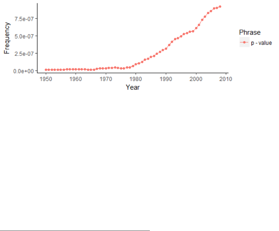
364
Figure 78. Graph indicating the continuously increasing popularity of p-values since
1950.
Note: Data was extracted from the Google Books Ngram corpus with the R package
“ngramr” (Lin et al., 2012).
We created a website which contains additional information on the logical fallacies
associated with NHST. The website is available under the following URL:
http://irrational-decisions.com/?page_id=441#nhst
To sum up this brief discussion of statistical methods, it can be concluded that NHST is
a methodological de facto standard which has been deeply implanted in the minds of
researchers over several generations. The critical facts about it are as old as its invention
(as the historical debate between Fischer versus Neyman/Pearson exemplifies). The
issue is not rational — it is irrational in nature. Most practicing researchers are not very
interested in discussing “nonpragmatic” statistical problems. They rather conform to the
predominant norm and use the methods that have been given to them and which are
regarded as the sine qua non for the field of research they work in (conformity might be
associated with a lack of introspective reflection, intrinsic motivation, and
epistemological curiosity, and perhaps scientific integrity, inter alia). Unconscious
motives play a pivotal role in this context as most decisions are not based on conscious
365
reflections but on unconscious processes. The problems associated with the use of p-
values are much more psychological and social than mathematics. P-values are deeply
ingrained in the methods of psychology, the bio-medical sciences, and countless other
scientific disciplines. The “Platonic-fallacy” is to assume that the decision which
inferential methods are utilised are based on rationality. The more complex the
discussed methods are from a mathematical point of view, the larger the divide between
System 1 (habitual) and System 2 processes (logic). The issue is thus psychological in
nature. We need to investigate why researchers are applying these methods in a
ritualistic non-reflective manner. What are their intentions and motivations. Indeed, it
can be argued that the p-ritual is reminiscent of OCD (Obsessive Compulsive Disorder)
symptomology and it would be interesting to investigate the comorbidity and whether a
significant proportion of the neural correlates are overlapping, e.g., dopaminergic
dysfunction in cortico-striatal-thalamic-cortical circuits (J. Wood & Ahmari, 2015).
The p-ritual has been institutionalised — consequently conformity to group norms and
obedience to authority play a central role. Moreover, the aforementioned systemic
incentive structure (i.e., publish or perish, the reliance on quantitative publication
indices to evaluate scholars, job insecurity, etc. pp.) play an important psychological
role in this context. It is not primarily a mathematical/logical problem but a
psychological/social one and the “extralogical factors” need to be addressed with the
same rigour if we want to tackle the current “statistical crisis” effectively. We argue that
“radical” measures need to be taken (the term radical is etymologically derived from the
Latin “radix” meaning “root”). That is, the root of the statistical crisis is primarily
psychological and not statistical (cf. G Gigerenzer, 1993) and therefore the root causes
need to be addressed instead of fruitless attempts to alleviate superficial
symptomological manifestations of the underlying issue. Recently, a new diagnostic
367
Table 37 have been proposed. Others have argued along the same lines — during the
development of the DSM-V it was ironically proposed that a “disorder covering
scientists addicted to questionable research practices” should be included in order to
deal with the “emerging epidemic of scientists engaging in questionable research
practices”. The following diagnostic criteria were formulated: “The essential feature of
pathological publishing is the persistent and recurrent publishing of confirmatory
findings (Criterion A) combined with a callous disregard for null results (Criterion B)
that produces a ‘good story’ (Criterion C), leading to marked distress in neo-Popperians
(Criterion D)” (Gullo & O’Gorman, 2012, p. 689). The “impact factor style of thinking”
(Fernández-Ríos & Rodríguez-Díaz, 2014) has been proposed as a new theoretical
framework which is pertinent in this context (viz., “assessing publications on the basis
of the impact factor”, “university policy habitus obsessed impact index”). Currently,
scientific content that has not been published in a journal that is indexed in impact
factor databases such as those underlying the Journal Citation Reports (JCR) is
academically not relevant. This has led to phenomena such as the “impact factor game”
and systematic impact factor manipulation (Falagas & Alexiou, 2008). The topic has
been discussed in some detail in a recent NATURE article entitled: “Beat it, impact
factor! Publishing elite turns against controversial metric” (E. Callaway, 2016).

368
Table 37
Potential criteria for the multifactorial diagnosis of “pathological publishing” (adapted
from Buela-Casal, 2014, pp. 92–93).
A. Having an excessive eagerness to show, disseminate, and advertise one’s
articles. This is reflected in a compulsive behaviour that consists of including
one’s publications and indicators of one’s publications in numerous devices that
are listed below.
B. Falsifying articles including false or manipulated data in articles to obtain more
publications or publish in journals with a higher impact factor.
C. Falsifying one’s CV including records of papers that are not such or duplicating
articles.
D. Distorting reality believing the data that one has falsified or manipulated.
E. Distorting reality believing that something is an article when it is not (e.g., book
reviews, meeting abstracts, editorial material, proceeding papers, notes). Internet
devices where indicators of publications are advertised:
1) ResearchGate
2) Scopus Author Identifier
3) WoS ResearcherID
4) Google Scholar profile
5) ORCID (Open Researcher and Contributor ID)
6) Twitter profile
7) Facebook profile
8) Linkedin profile
9) Mendeley profile
10) Delicious profile
11) Microsoft Academic Search profile
12) Academia.edu profile
13) CiteULike
14) Author Resolver™ (from Scholar Universe)
15) INSPIRE, the High Energy Physics information system
16) RePEc (Research Papers in Economics)
17) IraLIS (International Registry of Authors-Links to Identify Scientists).
18) Vivoweb profile
19) Blogger profile
20) Etc. pp.
F. Signing up for citation alerts
G. Really Simple Syndication (RSS)
H. Having e-mailing lists such as IweTel or Incyt
I. Calculating one’s h-index and updating it frequently
J. Counting citations to one’s work and updating the number frequently.
K. Counting article downloads
L. Calculating the cumulated impact factor and updating it frequently.

369
M. Publishing anything to increase the number of publications
N. Continuously updating one’s CV
O. Including one’s CV and various indicators of the CV in a personal web page.
P. Including ResearcherID or other indicators in web pages that include the
production of colleagues.
Q. Using Web 2.0 to increase the number of citations

370
In addition to systemic and psychological interventions which change the extrinsic
reinforcement schedule of academia and facilitate intrinsic motivation and altruistic
behaviour, we suggest that various Bayesian methods can be successfully combined
with preregistration
210
of studies (C. Chambers, 2013, 2014; McCarron & Chambers,
2015), a proposal which has previously been formulated in the context of
“neuroadaptive Bayesian optimization and hypothesis testing” (see Lorenz, Hampshire,
& Leech, 2017). Preregistration is a novel publishing initiative and provides an
important procedure that fosters transparency of research, mitigates publication bias,
and enhances the reproducibility of research results because researcher specify their
research strategies and planned hypothesis tests a priori before the research results are
disseminated which enhances trust in the research conclusions. That is, the underlying
motivation for conducting the study is explicitly disclosed prior to the analysis of the
data which counters illegitimate HARKing (HARK is a backronym for “Hypothesizing
After the Results are Known”) (Kerr, 1998) and the use of (unfortunately) pervasive
data mining techniques like a posteriori p-hacking as discussed earlier (i.e., data
dredging, data fishing, data snooping) (Head, Holman, Lanfear, Kahn, & Jennions,
2015; Simonsohn, 2014; Simonsohn, Nelson, & Simmons, 2014; Veresoglou, 2015).
210
Preregistration is the practice of publishing the methodology of experiments before they begin. This
strategy reduces problems stemming from publication bias and selective reporting of results.
See for example:
https://aspredicted.org/
https://cos.io/prereg/
https://www.psychologicalscience.org/publications/replication
A examplary list of currently preregistered studies can be found on Zotero:
https://www.zotero.org/groups/479248/osf/items/collectionKey/KEJP68G9
?

371
Figure 79. Questionable research practices that compromise the hypothetico-deductive
model which underpins scientific research (adapted from C. D. Chambers, Feredoes,
Muthukumaraswamy, & Etchells, 2014).
An excellent article on the topic published in AIMS NEUROSCIENCE is titled “Instead of
‘playing the game’ it is time to change the rules”. The recommended article is freely
available under the appended URL.
211
It is self-evident that such opportunist
research/analysis strategies as HARKing and p-hacking seriously compromise the
evolution, progress, veracity, and trustworthiness of science. Preregistration thus
prevents illegitimate post-hoc hypothesis testing procedures because hypotheses,
methods, and analysis protocols are prespecified prior to conducting the study. Another
key advantage of preregistration is that it enhances the quality of research due to an
initial external review of the research methodology (there are alternative preregistration
models which do not employ a review process (but see van ’t Veer & Giner-Sorolla,
211
Instead of “playing the game” it is time to change the rules: Registered Reports at AIMS Neuroscience
and beyond — https://orca.cf.ac.uk/59475/1/AN2.pdf
Generate
hypotheses
Design
study
Collect
data
Analyze
data
Interpret
data
Publish
results
Publication bias
Lack of openness
Lack of data sharing
Low statistical power
Lack of replication and cross-validation
372
2016)). Preregistration is a measure which attenuates the problem of publication bias
because information concerning statistically non-significant experiments becomes
available to the research community and can be utilised for meta-analytical research
purposes. That is, negative scientific results that are compatible with the null-hypothesis
can be published (after peer reviewed quality checks are met) without regard to an
arbitrary statistical significance threshold. However, it should be noted that
preregistration is not appropriate for purely exploratory research (e.g., exploratory
factor analysis using structural equation modelling, etc.), i.e., exploratory and
confirmatory analyses are complementary. Most statistical methods are only valid for
confirmatory research and are not designed for exploratory research and researchers
should therefore commit to a specific analytic technique prior to consulting the data.
With preregistration this crucial commitment is made before the data is collected. A
procedure which clearly enhances the credibility of research. In the same vein, it has
been argued that a stronger focus on confirmatory analyses reduces the “fairy tale
factor” in scientific research (E. J. Wagenmakers, Wetzels, Borsboom, van der Maas, &
Kievit, 2012). Hence, whenever a researcher wants to test prespecified
hypotheses/predictions preregistration is a highly recommended approach to enhance
the reliability, validity, veracity, and hence credibility of scientific research.
Preregistration is crucial in order to be able to demarcate “hypothesis testing” from
“hypothesis generation”, i.e., the oftentimes blurry distinction between prediction versus
postdiction.

373
Figure 80. Flowchart of preregistration procedure in scientific research.
In the psychological literature on reasoning and decision-making “hindsight-bias”
212
is a
widely studied phenomenon (Christensen-Szalanski & Willham, 1991; Hertwig,
Gigerenzer, & Hoffrage, 1997; Hoffrage et al., 2011; Pohl, 2007; Pohl, Bender, &
Lachmann, 2002; Roese & Vohs, 2012). Researchers are not immune to this ubiquitous
automatic cognitive bias (a System 1 process, to employ dual-systems terminology).
Consequently, it also applies to inferential decision-making in various statistical
research scenarios. Explicit awareness of the hindsight-bias (and multifarious other
cognitive biases which compromise reasoning) is thus of pivotal importance.
Consequently, researcher should be educated about the general internal workings of
their own minds (the instrument which does science). The well-documented psychology
of thinking and reasoning is of particular importance in this regard (Jonathan St B T
Evans, 2008; Kahneman, Slovic, & Tversky, 1982; K. E. Stanovich, 1999). However,
given the automatic nature of most cognitive biases, awareness is not sufficient because
prefrontally localised executive functions (System 2) which might help to regulate these
212
“Hindsight bias occurs when people feel that they “knew it all along,” that is, when they believe that
an event is more predictable after it becomes known than it was before it became known.“ (Roese &
Vohs, 2012, p. 411)
Publish
results
Analyze
Data
Collect
data
Design
Study
Preregister
374
automatisms are based on limited cognitive resources which are costly in physical
energetic terms, e.g., top-down regulation — glucose utilisation — ego-depletion
(Baumeister, Bratslavsky, Muraven, & Tice, 1998). Therefore, we need to implement
additional external systems which help to prevent such predictable fallacies.
Preregistration is a systematic procedural intervention which directly antagonises
unconscious biases which may distort scientific reasoning and decision-making (which
in turn forms the basis of many important real-world decisions). In a publication in the
Proceedings of the National Academy of Sciences, this novel trend has been termed
“The preregistration revolution” (Nosek, Ebersole, DeHaven, & Mellor, 2018).
Preregistration services (mainly web-based) are now becoming available for all
scientific disciplines and should soon be widely adopted by the general research
community.
6.11.2 The syllogistic logic of NHST
From a logical point of view NHST is based upon the logic of conditional syllogistic
reasoning (Cohen, 1994). Compare the following syllogisms of the form modus ponens:
Syllogism 1
1
st
Premise:
If the null hypothesis is true, then this data (D) cannot occur.
2
nd
Premise:
D has occurred.
Conclusion:
H
0
is false.
375
If this were the kind of reasoning used in NHST then it would be logically correct. In
the Aristotelian sense, the conclusion is logically valid because it is based on deductive
proof (in this case denying the antecedent by denying the consequent). However, this is
not the logic behind NHST. By contrast, NHST uses hypothetical syllogistic reasoning
(based on probabilisties), as follows:
Syllogism 2
1
st
Premise:
If H
0
is true, then this data (D) is highly unlikely.
2
nd
Premise:
D has occurred.
Conclusion:
H
0
is highly unlikely.
By making the major premise probabilistic (as opposed to absolute, cf. Syllogism 1) the
syllogism becomes formally incorrect and consequently leads to an invalid conclusion.
The following structure of syllogistic reasoning is implicitly used by many authors in
uncountable published scientific articles. This logical fallacy has been termed the “the
illusion of attaining improbability”. (Cohen, 1994, p.998).
376
Syllogism 3
1
st
Premise:
If H
0
is true, then this data (D) is highly unlikely.
2
nd
Premise:
D has occured
Conclusion:
H
0
is probably false.
Note: p(D|H
0
) ≠ p(H
0
|D)
6.11.3 Implications of the ubiquity of misinterpretations
of NHST results
Given that inferential statistics are at the very heart of scientific reasoning it is essential
that researchers have a firm understanding of the actual informative value which can be
derived from the inferential techniques they employ in order to be able to draw valid
conclusions. Future studies with academicians and PhD students from different
disciplines are needed to determine the “epidemiology” of these doubtless widespread
statistical illusions. The next sensible step would be to develop and study possible
systematic interventions and their effectiveness (but see Lecoutre et al., 2003). We
suggest that it is very necessary to invest in the development of novel pedagogical
concepts and curricula in order to teach the misleading logic behind NHST to students.
Moreover alternative statistical methods should be taught to students given that there is
no “magic bullet” or “best” inferential method per se. Gigerenzer (1993) points out that
“it is our duty to inform our students about the many good roads to statistical inference
that exist, and to teach them how to use informed judgment to decide which one to

377
follow for a particular problem” (p. 335). We strongly agree with this proposition. The
“new Bayesian statistics” (Kruschke & Liddell, 2017a) provide a viable alternative to
the Fisherian/Neyman-Pearsonian hybrid and researchers should be given the
appropriate training to be able to understand and sensibly utilise these powerful non-
frequentist methods.
6.11.4 P
rep
: A misguided proposal for a new metric of
replicability
We discussed the prevalent “replication fallacy” (G Gigerenzer, 1993) in the previous
section. In order to provide a genuine numerical indicator of replicability a new metric
called p
rep
has been proposed (Killeen, 2005b). Its primary objective is to provide an
estimate of replicability that does not involve Bayesian assumptions with regards to a
priori distributions of θ. The submission guidelines of the APA flagship journal
PSYCHOLOGICAL SCIENCE for some time explicitly encouraged authors to “use p
rep
rather
than p-values” in the results section of their articles. This fact is documented in the
internet archive,
213
a digital online-database that provides a mnemonic online system
containing the history of the web, a “digital time machine” (Rackley, 2009; Rogers,
2017). However, this official statistical recommendation by PSYCHOLOGICAL SCIENCE
has now been retracted (but the internet never forgets…). By default, the p
rep
metric is
based upon a one-tailed probability value of test statistic T (but it can be used for F-test
as well). However, this default can be changed into a two-tailed computation.
Equation 9. Formula to calculate P
rep
(a proposed estimate of replicability).
213
The URL of the relevant internet archive entry which documents the APA recommendation is as
follows.
https://web.archive.org/web/20060525043648/http://www.blackwellpublishing.com/submit.asp?ref=0956
-7976

378
rep
= [1 + (
1
)
]
The mathematical validity of p
rep
has been seriously called into question (Doros &
Geier, 2005). Based on the results of simulation studies, it has been convincingly argued
that “p
rep
misestimates the probability of replication” and that it “is not a useful statistic
for psychological science” (Iverson, Lee, & Wagenmakers, 2009). In another critical
reply to Killeen’s proposal, it has been suggested that hypothesis testing using Bayes
factor analysis is a much more effect strategy to avoid the problems associated with
classical p-values (E.-J. Wagenmakers & Grünwald, 2006). One of the main
shortcoming of the suggested new metric is that p
rep
does not contain any new
information ‘over and above’ the p-value — it is merely an extrapolation. Another
weakness is that a priori information (for example knowledge from related previous
studies) cannot be incorporated. Killeen responds to this argument with the "burden of
history argument”, i.e., each result should be investigated in isolation without taking
any prior knowledge into account (viz., he advocates uniform priors). However, on
logical grounds it is highly questionable whether a single study can be used as a basis
for estimating the outcome of future studies. Various confounding factors (e.g., an
unanticipated tertium quid) might have biased the pertinent results and consequently
lead to wrong estimates and predictions. According to aphoristic “Sagan standard”:
Extraordinary claims require extraordinary evidence.
214
The novel p
rep
metric does not
align with this Bayesian philosophy. From our point of view, the main advantage to
report and discuss p
rep
is that it helps to explicate and counteract the ubiquitous
“replication fallacy” (G Gigerenzer, 2004) associated with conventional p-value. The
replication fallacy describes the widespread statistical illusion that the p-value contains
214
Pierre-Simon Laplace formulated the same proportional principle: „The weight of evidence for an
extraordinary claim must be proportioned to its strangeness“ (Flournoy, 1899).

379
information about the replicability of experimental results. In our own survey at a
CogNovo workshop the “replication fallacy” was the most predominant
misinterpretations of p-values. 77% (i.e., 14 out of 18) of our participants (including
lecturers and professors) committed the replication fallacy. Only one participant
interpreted the meaning of p-values correctly, presumably due to random chance. In a
rejoinder titled “Replicability, confidence, and priors” (Killeen, 2005b) Killeen
addresses several criticisms in some detail, particularly with regards to the stipulated
nescience
215
of δ. Indeed, it has been argued that “replication probabilities depend on
prior probability distributions” and that Killeen's approach ignores this information and
as a result, “seems appropriate only when there is no relevant prior information”
(Macdonald, 2005). However, in accordance with the great statisticians of this century
(e.g., Cohen, 1994, 1995; Meehl, 1967), we argue that the underlying syllogistic logic
of p-values is inherently flawed and that any attempt to rectify p-values is moribund. It
is obvious that there is an urgent and long due “need to change current statistical
practices in psychology” (Iverson et al., 2009). Creative change and innovation is vital
to resolve the “statistical crisis” (Gelman & Loken, 2014; Loken & Gelman, 2017b).
The current academic situation is completely intolerable and the real-world
ramifications are tremendously wide and complex. New and reflective statistical
thinking is urgently needed, instead of repetitive “mindless statistical rituals”, as Gerd
Gigerenzer
216
put it (G Gigerenzer, 1998, 2004). However, deeply engrained social
215
In the semantic context at hand, nescience (etymologically derived from the Latin prefix ne "not" +
scire "to know" cf. science) means “lacking knowledge” which is a more appropriate term than ignorance
(which describes an act of knowingly ignoring). Unfortunately, linguistic diversity is continuously
declining. A worrisome trend which is paralleled by a loss of cultural and biological diversity (Maffi,
2005; Worm et al., 2006b), inter alia.
216
Gigerenzer is currently director of the “Center for Adaptive Behavior and Cognition” at the Max
Planck Institute in Berlin. In his article entitled “Mindless Statistics” Gigerenzer is very explicit with
regards to the NHST ritual: “It is telling that few researchers are aware that their own heroes rejected
what they practice routinely. Awareness of the origins of the ritual and of its rejection could cause a
virulent cognitive dissonance, in addition to dissonance with editors, reviewers, and dear colleagues.

380
(statistical) norms are difficult to change, especially when large numbers of researchers
have vested interests to protect the prevailing methodological status quo as they were
predominantly exclusively trained in the frequentist framework (using primarily the
proprietary software IBM® SPSS). Hence, a curricular change is an integral part of the
solution. Statistical software needs to be flexible enough to perform multiple
complementary analysis. Until recently, SPSS did not provide any modules for
Bayesian analyses even though the IBMs developers could have easily implemented
alternative statistical methods to provide researchers with a more diverse statistical
toolbox. Open-source software clearly is the way forward. The open-source community
is highly creative and innovative. For instance, CRAN now host < 10000 packages for
R and all kinds of sophisticated analyses can be conducted within the R environment.
IBM is aware of the rise of open-source software (which is obviously seen as a fierce
competitor for market shares). Presumably in reaction to the changing economic
pressures, SPSS is now able to interface with R and Bayesian methods are now
becoming available for the first time. Moreover, Markov chain Monte Carlo methods
will become available in future versions of SPSS. All of this could have been realised
much earlier. However, given the rapid upsurge of R, SPSS is now practically forced to
change its approach towards (i.e., exnovation) in order to defend market shares (a
passive/reactive approach, i.e., loss aversion (Novemsky & Kahneman, 2005)).
To conclude this important topic, it should be emphasised that rational approaches vis-
à-vis problems associated with replicability, confidence, veracity, and the integration of
prior knowledge are pivotal for the evolution and incremental progress of science. It is
obvious that the fundamental methods of science are currently in upheaval.
Suppression of conflicts and contradicting information is in the very nature of this social ritual.” (G
Gigerenzer, 2004, p. 591)

381
6.11.5 Controlling experimentwise and familywise α-
inflation in multiple hypothesis testing
In our experiments we tested several statistical hypotheses in a sequential manner.
Whenever a researcher performs multiple comparisons, α-error control is of great
importance
217
(Benjamini & Braun, 2002; Benjamini & Hochberg, 1995a; Holland &
Copenhaver, 1988; Keselman, Games, & Rogan, 1979; Seaman, Levin, & Serlin, 1991;
Simes, 1986; Tukey, 1991). However, empirical data indicates that most researchers
completely neglect this important statistical correction (Nuijten, Hartgerink, van Assen,
Epskamp, & Wicherts, 2016b). An α-error (also known as “Type I error”) occurs when
a researcher incorrectly rejects a true null hypothesis. On the other hand, a β-error
(“Type II error”) is inversely related to the probability of committing an α-error, i.e.,
incorrect acceptance of a false null hypothesis (see
217
This does not apply to Bayesian hypothesis testing and parameter estimation approaches.
382
Table 38). In every situation in which multiple tests are performed the α-error rate is
inflated in proportion to the number of hypothesis tests performed. R.A. Fisher
discussed this central problem in his seminal book The Design of Experiments (R. A.
Fisher, 1935), which laid the foundation for modern statistical hypothesis testing as
utilised in the majority of scientific and bio-medical disciplines. He proposed the “Least
Significant Difference” (LSD) procedure in order to counteract α-inflation (L. J.
Williams & Abdi, 2010). LSD has been criticized for not being conservative enough in
many situations and its “liberalness” has been demonstrated in mathematical simulation
experiments (using Monte Carlo methods) which specifically focused on pairwise
comparisons of two means (Boardman & Moffitt, 1971). Since Fisher’s early attempt,
countless alternative multiple comparison error rate control procedures have been
invented (inter alia Abdi, 2007; O. J. Dunn, 1961; Holm, 1979; Hommel, 1988; Seaman
et al., 1991; Simes, 1986). For a comprehensive review see (Holland & Copenhaver,
1988).
The issue is particularly pertinent in scientific disciplines that deal with vast numbers of
simultaneous comparisons, for instance, in genetics (e.g., genome-wide association
studies, conservation genetics, etc.) (Moskvina & Schmidt, 2008; Narum, 2006).
However, even if a researcher tests only two hypotheses, α-error has to be considered,
otherwise subsequent logical inferential conclusions might be biased/invalid. To
illustrate the general point that statisticians need to explicitly integrate potential sources
of error in their analytic efforts Leslie Kish aptly adapted one of Alexander Popes heroic
couplets: "To err is human, to forgive divine but to include errors in your design is
statistical." (Kish 1978).

383
Table 38
Hypothesis testing decision matrix in inferential statistics.
Classification of hypothesis-testing
decisions
Truth-value of H
0
True
False
Decision about H
0
Reject
α
(False Positive)
False interference
1- α
(True Positive)
Correct inference
Fail to reject
1- β
(True Negative)
Correct inference
β
(False Negative)
False interference
Note. The Latin-square is isomorphic to the payoff matrix in a legal case, viz., juridical
decision-making. The defendant might be guilty or innocent and the judge might decide
to sentence the defendant or not.
The appropriate level of significance in relation to the number of comparisons is of
direct practical relevance for the research at hand. We conducted a series of experiments
(4 of which are reported here) and each experiment consisted of 2 hypothesis tests.
Summa summarum, this results in a total of 8 hypothesis tests. Because we had specific
a priori predictions we avoided omnibus F-tests, otherwise the number would be even
higher. A crucial question is the following: Should one control the experimentwise error
rate or the familywise error rate? There are many techniques to correct for multiple
comparisons, some of them are statistically more conservative and some are more

384
liberal. If one would apply a simple stepwise Bonferroni correction (experimentwise) to
the current analyses, the α-level would be divided by the number of comparisons per
experiment. If one applies a classical Bonferroni correction this results in a p-value of
0.05 / 8 = 0.00625. In other words, one should only reject H
0
(i.e., results are only
declared as statistically significant) if p < 0.00625. If one would like to control for the
familywise error rate the calculation becomes more complex. We will discuss some of
the details in the following section.
The familywise error rate defines the probability of making at least one α-error.
FWER = (1) where is the number of α-errors.
Equation 10: Holm's sequential Bonferroni procedure (Holm, 1979).
()
>
+ 1
The Holm-Bonferroni method ensures that FWER , i.e., it allows the researchers to
ensure that the probability of committing one or more α-errors stays below an arbitrary
threshold criterion (conventionally α = 0.05 but this decision-threshold can/should be
adjusted according to circumstances, e.g., based on a cost-benefit analysis).
• The following example illustrates the procedure:
• Conventional significance level α = 0.05
• smallest P-value: α1 = α/k
• next smallest P-value: α2 = α/(k-1)
• next smallest P-value: α3 = α/(k-2)
• halting-rule: stop at first non-significant α- value
385
Let
, … ,
denote a family of hypotheses and
, . . . ,
the p-values that were
computed after a given experiment has been conducted.
()
…
()
1. Significance levels are ordered ascendingly, e.g.:
p-value
0.00001
0.00099
0.00300
0.03500
0.05000
2. The number of tests is quantified:
p-valuek
0.00002 1
0.00081 2
0.00337 3
0.03666 4
0.05000 5
386
3. The number of tests is arranged in an inverse order
p-value k k
-1
0.00002 1 5
0.00081 2 4
0.00337 3 3
0.03666 4 2
0.05000 5 1
4. The respective significance level is divided by the inverse
p-value k k
-1
adjusted p-value
0.00002* 1 5 0.05/5=0.01
0.00081* 2 4 0.05/4=0.0125
0.00337* 3 3 0.05/3=0.016667
0.03666 4 2 0.05/2=0.025
0.05000 5 1 0.05/1=0.05
5. According to Holm's sequential Bonferroni procedure the first three p-values are
regarded as significant because they are smaller than the corresponding adjusted p-
value, i.e., p < adjusted p.
Holm's sequential Bonferroni procedure ensures that the family wise error rate (FWER)
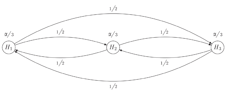
387
From a statistical point of view, this multiple test procedures is a subclass of so called
“closed testing procedures” which entail various methodological approaches for
performing multiple hypothesis tests simultaneously.
Figure 81. Graphical illustration of the iterative sequential Bonferroni–Holm procedure
weighted (adapted from Bretz, Maurer, Brannath, & Posch, 2009, p. 589).
Figure 81 illustrates a Bonferroni-Holm procedure with = 3 hypotheses and an initial
allocation of = (/3, /3, /3). Each node corresponds to an elementary hypothesis
and the associative connections are directional and weighted.

388
Alternative methods for α-control include the Dunn–Šidák correction (Šidák, 1967) and
Tukey's honest significance test (Tukey, 1949), inter alia. The associated formulae are
given below.
Equation 11: Dunn-Šidák correction (Šidák, 1967)
= 1 (1 )
Equation 12: Tukey's honest significance test (Tukey, 1949)
=
Interestingly, a recent paper published by Nature (Benjamin et al., 2017) argues for the
radical modification of the statistical threshold (in a collective effort numerous authors
propose to change the p-value to 0.005). We argue that the adjustment of p-values for
multiple comparisons is at least equally important and it has been shown that
researchers generally do not correct for multiple comparisons (Nuijten et al., 2016a).
Besides the experimentwise adjustment, the familywise error rate adjustment is even
more rarely reported in publications, even though it is at least of equal importance.
Multiple comparisons techniques form an integral part of empirical research. However,
they confront researchers with deep philosophical as well as pragmatic problems
(Tukey, 1991). Current academic incentive structures put researchers under “enormous
pressure to produce statistically significant results” (Frane, 2015, p. 12). It follows that
methods that reduces statistical power are not necessarily welcomed by the research
community. A recent paper titled “Academic Research in the 21st Century: Maintaining
Scientific Integrity in a Climate of Perverse Incentives and Hypercompetition”
(Edwards & Roy, 2017) addresses several relevant systemic issue in more detail.
389
Experimentwise and familywise error control techniques are incongruent with the
“publish or perish” (Rawat & Meena, 2014) and “funding or famine” (Tijdink, Verbeke,
& Smulders, 2014) mentality imposed on many researchers. If researchers would
appropriately utilise statistical methods that substantially reduce α-levels, then they put
themselves in a competitive disadvantage (even though the decision to reduce α might
be completely rational on logical and statistical grounds). Given that academia is often
displayed as a competitive environment, evolutionary principles apply. Academic
fitness is closely linked to the number of papers a researcher has published. In an
academic climate of hypercompetition, quantitative metrics predominantly determine
administrative decision making (Abbott et al., 2010). Specifically, the “track record” of
researchers is largely evaluated quantitatively, i.e., researchers are ranked according to
the number of publications and the impact factors of the journals they have published in.
This leads to publication pressure and the phenomenon of “p-hacking” has become a
topic of substantial interest in this context (Bruns & Ioannidis, 2016; Head et al., 2015;
Veresoglou, 2015). It has been pointed out that the prevailing academic incentive
structures implicitly reinforce unethical behaviour and academic misconduct (Edwards
& Roy, 2017). In the context of hypothesis testing, the last thing an intrinsically
motivated and career-oriented researchers want to learn about are methods that decrease
statistical power (independent of the logical foundation of these methods). It is
important to recall that hypothesis testing is based on the Popperian logic of
falsification. However, it seems as if the logical foundations of hypothesis testing have
been almost forgotten. Negative results are almost impossible to publish (Borenstein,
Hedges, Higgins, & Rothstein, 2009; Franco, Malhotra, & Simonovits, 2014; Mathew &
Charney, 2009; Nuijten et al., 2016b). In order to facilitate the publication of negative
result, a special journal was invented: “The Journal in support of the null hypothesis”.

390
However, a single journal cannot counterbalance the publication bias which is
associated with the strong emphasis on significant results. Lowering the p-value
threshold (as has been suggested by a large group of influential researchers (Benjamin
et al., 2017; cf. Chawla, 2017))) is therefore also no solution to the “cult of significance
testing”
218
. Instead, we need to reconsider the logical fundamentals of the scientific
method and how they are implemented in the sociology of science.
Instead of trying to refute their hypotheses, researchers currently largely try to confirm
them. This cognitive bias is well-known in the psychology of thinking and reasoning
and belongs to the class of “confirmation biases” (M. Jones & Sugden, 2001;
Nickerson, 1998; Oswald & Grosjean, 2004), which have been documented in diverse
areas, for instance in the context of psychiatric diagnostic decision making (Mendel et
al., 2011), financial investments (Park, Konana, & Gu, 2010), and visual search (Rajsic,
Wilson, & Pratt, 2015), inter alia. However, this (confirmatory) approach towards
hypothesis testing stands in sharp contrast with the Popperian logic of hypothesis
testing, i.e., falsification. In his books “The Logic of Scientific Discovery” (Popper,
1959) and later in “Conjectures and Refutations: The Growth of Scientific Knowledge”
(Popper, 1962) Popper advocated the concept of “bold hypotheses”. According to
Popper the growth of scientific knowledge is achieved by means of articulating bold
hypotheses (conjectures), and consequently trying to experimentally refute (falsify)
them. It is a logical impossibility to conclusively proof a given hypothesis (e.g., all
swans are white). Science can only try to falsify (e.g., search for the one black swan in
the universe). Hence, researchers should not seek support for their hypotheses, they
should try to refute them by all means possible. However, in reality researchers have
218
The informative book with the fitting title “The cult of significance testing” discusses how significance
testing dominates many sciences, i.e., researchers in a broad spectrum of fields, ranging from the zoology,
biomedical sciences, to neuroscience, to psychology, etc. pp. employ the p-ritual.

391
vested interest (they are not as objective and neutral as science would demand them to
be) and it as has been famously pointed out by Imre Lakatos in his seminal paper titled
“The role of crucial experiments in science” that in practice scientists try to confirm
their hypotheses and do not adhere to falsificationism (Lakatos, 1974).
Falsifiability is a defining demarcation-criterion in Poppers framework which separates
“science” from “pseudo-science”. A hypothesis which cannot be falsified (e.g., God is
love) is not a scientific statement. We argue that null results are at least as important as
positive results (if not more so) and we are convinced that editorial policies need to
change. Otherwise scientific progress will continue to be seriously impeded. The
following parable illustrates the importance of negative results intuitively:
There's this desert prison, see, with an old prisoner, resigned to his life, and a young
one just arrived. The young one talks constantly of escape, and, after a few months, he
makes a break. He's gone a week, and then he's brought back by the guards. He's half
dead, crazy with hunger and thirst. He describes how awful it was to the old prisoner.
The endless stretches of sand, no oasis, no signs of life anywhere. The old prisoner
listens for a while, then says, Yep, I know. I tried to escape myself twenty years ago. The
young prisoner says, You did? Why didn't you tell me, all these months I was planning
my escape? Why didn't you let me know it was impossible? And the old prisoner shrugs,
and says, So who publishes negative results? (Hudson, 1968, p. 168)
Currently most authors, editors, reviewers and readers are not interested in seeing null
results in print. Based on the Popperian logic of falsification
219
, null results are
important contributions to the corpus of scientific knowledge. The currently prevailing
219
However, Popper ideas are widely misunderstood and his falsificationism is often reduced to be
falsifiability (Holtz & Monnerjahn, 2017). A closer reading of Popper would prevent this
misinterpretation.

392
publication bias (aka. “the file drawer effect” because negative results end up in the file-
drawer) is a serious problem which needs to be addressed. Moreover, the proportion of
replication studies is minute, that is, almost no published finding is ever replicated as
replication is not reinforced. All other statistical considerations (Bayesian vs.
frequentists, exact α, correction for multiple comparison, replicability, etc. pp.) are
secondary. As long as this fundamental issue is not solved, science cannot call itself
rational. Thus far, we have not encountered a single valid argument which justifies the
exclusive focus on positive (confirmatory) results.
In addition, the correct adjustment of α-levels is a logical prerequisite for valid
inferences and conclusions (that is, in the NHST framework). However, if stringent
(appropriate) α-control techniques would be applied, many experiments would not reach
statistical significance at the conventional α level (and hence would not get published).
This also applies to the “institution-wide error rate”
220
, that is the total number of
hypotheses which are tested within a given institution over a given period of time. In
other words, if researchers within a given institution would apply more conservative
criteria, the ranking of the institution would suffer (the ranking is based on research
metrics like the total number of publications). It can be seen, that many extraneous
illogical factors prevent research from applying proper statistical error correction
methods, independent of their logical validity. We term these factors “extralogical
factors” in order to emphasise their independence from purely rational scientific
considerations. We argue that extralogical factor seriously impede scientific progress
220
The “institution-wide error rate” is a term invented by the author to refer to the total number of
hypotheses tested in a given academic institution. The more hypotheses are tsted, the higher the
probability that the institution will publish large numbers of papers which are based on statistically
significant results (a key factor for the ranking of the institution and hence for funding). Ergo, institutions
might encourage large numbers of studies with multiple hypotheses tests per study in order to gain a
competitive advantage in the competition for limited resources (a quasi-Darwinian strategy).
393
and that they compromise scientific integrity. Furthermore, we argue that interpersonal
personality predispositions play an important role in this scenario. Intrinsically
motivated researchers focus less on external reinforcement and are more focused on
knowledge and accuracy as an inherent intrinsic reward (Sorrentino, Yamaguchi, Kuhl,
& Keller, 2008). By contrast, extrinsically motivated researchers are primarily
motivated by external rewards. It follows, that under the prevailing reinforcement
schedule, intrinsically motivated researchers are in a disadvantaged position, even
though their virtuous attitudes are most conducive to scientific progress (Kanfer, 2009;
Maslow, 1970). Unfortunately, economic interests dominate academia, a phenomenon
Noam Chomsky termed “the corporatization of the university” (Chomsky, 2011) and
the ideals of Humboldtian science and education (Hanns Reill, 1994) (e.g., corporate
autonomy of universities, holistic academic education) are currently largely supplanted
by the military-industrial-entertainment complex (see Chomsky, 2011) and the
associated Taylorism (Littler, 1978).
In his analysis “how America's great university system is being destroyed”, Chomsky
points out that faculty are increasingly hired on the Walmart model” (Punch &
Chomsky, 2014). This has obviously implications for the conduct of researchers. If
publication metrics are a crucial factor which determines job-security and promotion,
then the prevailing incentive contingencies reinforce a focus on self-serving motives
which might be incompatible with scientific virtuous which require an altruistic
orientation (Edwards & Roy, 2017). The behavioural effects of the prevailing
reinforcement contingencies can be largely accounted for in a simple behaviouristic S-R
model.
For an extended discussion of this extremely important problem see the article by
Henry Steck (2003) entitled “Corporatization of the University: Seeking Conceptual

394
Clarity” published in “The Annals of the American Academy of Political and Social
Science”. The article concludes: “To the extent that a corporatized university is no
university or corporate values are not academic values … it is the burden for faculty to
address the issue of protecting traditional academic values” (p.66). Several insightful
books have been published on this topic by Oxford (Ginsberg, 2011) and Harvard
(Newfield, 2008) University Press, inter alia. The following books provide an in-depth
analysis of the situation:
• “Neoliberalism and the global restructuring of knowledge and education” (S. C.
Ward, 2012),
• “Global neoliberalism and education and its consequences” (Hill & Kumar,
2009),
• “On Miseducation” (Chomsky & Macedo, 2000)
• “Manufacturing Consent: Noam Chomsky and the Media” (Chomsky, 1992)
Relevant articles include:
• “Educating consent? A conversation with Noam Chomsky on the university and
business school education” (P. Fleming & Oswick, 2014)
• “Neoliberalism, higher education and the knowledge economy: From the free
market to knowledge capitalism” (Olssen & Peters, 2005)
In this context, we also recommend a review of Edward Bernays’ classical work which
is important for a basic understanding of mass-psychology (E. L. Bernays, 1928,
1936)
221
.
221
Bernays was a nephew of Sigmund Freund who applied psychoanalytic principles to the public domain
(i.e., mass psychology). Bernays is often called the called “the father of public relations” and also “the

395
This “neo-liberal” shift in academic values and priorities has ramifications for the
foundations of science which cannot be underestimated. When universities compete on
a “free market” for funding (based on ranking positions) on the basis of the number of
publications, α-error control techniques which would limit the output of publications are
a topic which is unconsciously or consciously avoided for obvious reasons. For instance
“universities have attempted to game the system by redistributing resources or investing
in areas that the ranking metrics emphasize” (Edwards & Roy, 2017, p. 54). Related
sociological research examined “how and why the practice of ranking universities has
become widely defined by national and international organisations as an important
instrument of political and economic policy” (Amsler & Bolsmann, 2012).
The reader might question the relevance of this discussion for the research at hand. In
anticipation of such an objection we would like to accentuate that these considerations
are of practical importance for the calculations of significance levels in the current
experiments. Besides, they have real-world implication for the way in which null results
are reported (or ignored). Recall the so called “file-drawer effect” (a.k.a. “publication
bias”) which systematically distorts the validity and reliability of scientific inferences
because negative results are not reported in the literature (Asendorpf & Conner, 2012;
Borenstein et al., 2009; Kepes, Banks, McDaniel, & Whetzel, 2012; Mathew &
Charney, 2009; Møllerand & Jennions, 2001; Jeffrey D. Scargle, 1999; Thornton & Lee,
2000).
father of spin” (L’Etang, 1999). Bernays was a pioneer in the field of propaganda and he coined the term
in his eponymous book (E. L. Bernays, 1928). Propaganda is mainly concerned with what Chomsky calls
“the manufacturing of consent” (Chomsky, 1992). The discipline which focuses on mass-psychology (i.e.,
the systematic manipulation of the masses) was later euphemistically renamed into “public relations”
(Ihlen & van Ruler, 2007) after the Nazis “spoiled” the terminus propaganda (Joseph Goebbels was a
student of Bernays work).
396
6.11.6 α-correction for simultaneous statistical inference:
familywise error rate vs. per-family error rate
A meta-analysis of more than 30000 published articles indicated that less than 1%
applied α-corrections for multiple comparisons even though the median number of
hypothesis tests per article was ≈ 9 (Conover, 1973; Derrick & White, 2017; Pratt,
1959). A crucial, yet underappreciated difference, is the distinction between 1) the
familywise (or experimentwise) error rate (FWER), and 2) the per-family error rate
(PFER). FWER is the probability of making at least one Type I error in a family of
hypotheses. The PFER, on the other hand, which is the number α-errors expected to
occur in a family of hypotheses (in other words, the sum of the probabilities of α-errors
for all the hypotheses in the family).The per-comparison error rate (PCER) is the
probability of a α-error in the absence of any correction for multiple comparisons
(Benjamini & Hochberg, 1995b). Moreover, the false discovery rate (FDR) quantifies
the expected proportion of "discoveries" (rejected null hypotheses) that are false
(incorrect rejections).
The majority of investigations focus on the former while the latter is largely ignored
even though it evidently is at least equally important if not more so (Barnette & Mclean,
2005; Kemp, 1975). The experimentwise (EW) error rate does not take the possibility of
multiple α -errors in the same experiment into account. Per-experiment (PE) α-control
techniques control α for all comparisons (a priori and post hoc) in a given experiment.
In other terms, they consider all possible α-errors that in a given experiment. It has been
persuasively argued that per-experiment α control is most relevant for pairwise
hypothesis decision-making (Barnette & Mclean, 2005) even though most textbooks
(and researchers) focus on the experimentwise error rate. Both approaches differ
significantly in the way they adjust α for multiple hypothesis tests. It has been pointed
397
out that the almost exclusive focus on experimentwise error rates is not justifiable
(Barnette & Mclean, 2005). From a pragmatic point of view, per-experiment error
correction is much closer aligned with prevailing research practices. In other words, in
most experiments it is not just the largest difference between conditions which is of
empirical interest and most of the time all pairwise comparisons are computed. The EW
error rate treats each experiment as one test even though multiple comparisons might
have been conducted. A systematic Monte Carlo based comparison between four
different adjustment methods showed that, for experimentwise control, Tukey’s HSD is
the most accurate procedure (as an unprotected test). If experimentwise α-control is
desired, Tukey’s HSD (unprotected) test is the most accurate procedure. If the focus is
on per-experiment α-control, the Dunn-Bonferroni (again unprotected) is the most
accurate α-adjustment procedure (Barnette & Mclean, 2005).
6.11.7 Protected versus unprotected pairwise comparisons
In anticipation of the objection why we conducted unprotected comparisons
straightway, we will discuss the use of protected vs. unprotected statistical tests in some
detail. It is generally regarded as “best practice” to compute post hoc pairwise multiple
comparisons only after a significant omnibus F-test. Many widely sold textbooks either
explicitly or implicitly advocate the utilisation of protected tests before post hoc
comparisons are conducted (i.a., Kennedy & Bush, 1985; Maxwell & Delaney, 2004).
That is, a 2-stage strategy is advocated and widely adopted by most researchers as
evidenced in the literature. The 2-stage strategy makes post hoc pairwise comparisons
conditional on a statistically significant omnibus F-test (hence the name protected test).
However, this recommendation is not evidence based and there is no analytic or
empirical evidence in support of this practice. To the contrary, it has been empirically

398
demonstrated that this strategy results in a significant inflation of α-error rates
(Keselman et al., 1979). Further empirical evidence against the 2-stage (protected)
testing strategy is based on a Monte Carlo analysis which explicitly compared protected
versus unprotected testing procedures. Independent of the error control method used
(i.e., Dunn-Šidák, Dunn-Bonferroni, Holm, Tukey’s HSD) unprotected tests performed
significantly better compared to protected tests (Barnette & Mclean, 2005). This
simulation study clearly demonstrated that using the F-test as a “protected gateway” for
post hoc pairwise comparison is overly conservative. The simulation results clearly
show that protected tests should not be used. Independent of weather experimentwise or
per-experiment α-control is used, and no matter which α-error control technique is used
(i.e., Dunn-Šidák, Dunn-Bonferroni, Holm, Tukey’s HSD, etc.) unprotected tests
generally outperformed their protected counterparts.
222
Based on this evidence, it can be
safely concluded that unprotected testing procedures should be preferred over 2-stage
protected procedures. The conventional wisdom of conducting omnibus tests before
post hoc comparisons are performed does not stand the empirical/mathematical test. The
authors of the previously cited Monte Carlo simulation study conclude their paper with the
following statement: “
Only when one is willing to question our current practice can one
be able to improve on it” (Barnette & Mclean, 2005, p. 452).
6.11.8 Decentralised network systems of trust: Blockchain
technology for scientific research
An interesting and innovative proposal is to use blockchain technologies (usually
associated with digital crypto currencies like, for instance, Bitcoin or Ethereum) to
222
A neglectable exception was only the Holm procedure in the case of per-experiment error control (but
not in the case of experimentwise error control). In this specific constellation, α of .10 was more accurate
as a protected test as compared to an unprotected test. This accuracy difference was lower when α was .05
or .01.
399
counteract the replication crisis, to validate empirical findings, and to improve and
optimize the scientific procedure on a large scale (Bartling & Fecher, 2016). The
authors suggest that “Blockchain could strengthen science's verification process,
helping to make more research results reproducible, true, and useful” (Bartling &
Fecher, 2016, p. 1). Even though this proposal might seem unrealistic or overstated to
those unfamiliar with blockchain technologies, we think that this is indeed an excellent
innovative and creative proposal because blockchain technologies can be used in all
situations which require a high degree of trust. In other words, it is a decentralised
(distributed) technology which is useful in many scenarios in which trust is of central
concern and it has been predicted that the “blockchain revolution” (Tapscott &
Tapscott, 2016a) will influence not only online transactions, but that it will profoundly
change many aspects of society which go far beyond financial services (Foroglou &
Tsilidou, 2015; Grech & Camilleri, 2017; Idelberger, Governatori, Riveret, & Sartor,
2016; Tapscott & Tapscott, 2016b). Given that the replication crisis challenges the
trustworthiness of scientific data, blockchain seems to be a potential candidate which
should be carefully considered in this respect. The Economist called the blockchain “the
trust machine” (TheEconomist, 2015). Trust “is hardcoded in the Blockchain protocol
via a complex cryptographic algorithm” (Benchoufi & Ravaud, 2017). For instance,
blockchain-timestamped protocols have been suggested to improve the trustworthiness
of medical science (Irving & Holden, 2017). Moreover, the use of blockchain
technologies has been suggested to improve clinical research quality where
“reproducibility, data sharing, personal data privacy concerns and patient enrolment in
clinical trials are huge medical challenges for contemporary clinical research”
(Benchoufi & Ravaud, 2017). Based on these proposals and the intrinsic trustworthiness
of the implemented cryptographic algorithms, it can be convincingly argued that
400
innovative decentralised blockchain networks might become of central importance to
the scientific endeavour. Specifically, it might provide a cryptographic/mathematical
basis for transparent, unbiased, and decentralised scientific research of the future. We
propose the phrase “the digital decentralisation of science”. An improvement of a part
of the system which underlies the scientific method which only became available when
sufficient computational resources became available. The decentralised nature of the
system is characteristic of a general tendency towards distribution, openness, and
transparency. Science and trust are obviously closely interlinked concept. Therefore,
science needs to be implemented in an and ideological and technological system which
intrinsically support this virtuous feature which lies at the very heart of science.
Namely: Trust. In a sense, code is morality, i.e., code defines the laws under which a
system operates. The current centralised publishing landscape and the associated
editorial policies have all kinds of inherent procedural biases and the
selectivity/publications-bias which lies at the core of the replicability crisis is just one of
the many manifestations and consequences that impede and compromise the
trustworthiness, integrity, and authenticity of the scientific endeavour. Openness and
decentralisation is the way forward (Bohannon, 2016; McKenzie, 2017; Perkel, 2016).
401

402
6.12 Potential future experiments
6.12.1 Investigating quantum cognition principles across
species and taxa: Conceptual cross-validation and
scientific consilience
Decision-making is not unique to human primates and has been demonstrated in various
animal species (Steven, 2010; A. J. W. Ward, Sumpter, Couzin, Hart, & Krause, 2008),
plants (Schmid, 2016), fungi/moulds (Tero et al., 2010), bacteria (Z. Xie, Ulrich,
Zhulin, & Alexandre, 2010), viruses (Weitz, Mileyko, Joh, & Voit, 2008), at the cellular
level (Perkins & Swain, 2009), and even in single photons (Naruse et al., 2015).
Fascinatingly, there appear to exist some astonishing generalities between the decision-
making principles that govern these multifarious domains (e.g., Ben-Jacob, Lu, Schultz,
& Onuchic, 2014). It would be highly interesting to investigate noncommutativity and
constructive principles in completely different domains in order to establish scientific
consilience.
223
Are bacterial decisions noncommutative? Are the decisions made by
fungal mycelia constructive in nature? Do photobiological processes in various species
follow the same principles as human visual perception? If scientific evidence would
affirm these research questions this kind of “concordance of evidence” would underline
the robustness and generalizability of quantum probability decision-making principles.
Scientific consilience
The strength of evidence increases when multiple sources of evidence converge. This
has also been termed the “unity of knowledge” (E. O. Wilson, 1998a). Consilience is
based on the utilisation of unrelated research methodologies and measurement
223
The etymological root of the word consilience is derived from the Latin consilient, from com "with,
together" and salire "to leap, to jump," hence it literally means “jumping together” (of knowledge).
403
techniques. In other words, the research approaches are relatively independent. The
generalisability and robustness of converging evidence for a specific logical conclusion
is based on the number of different research approaches in support of the conclusion.
Furthermore, if equivalent conclusions are reached from multiple perspectives this
provides evidence in support of the reliability and validity of the utilised research
methodologies themselves. Resilience reduces the impact of confounding factors (e.g.,
method related measurement errors) because these errors do not influence all research
methods equally. Resilience thus “balances-out” method specific confounds. The same
principle also applies to logical confounds (e.g., logical fallacies and biases). In the
philosophy of science, this has been termed “consilience of inductions” (Fisch, 1985;
Hesse, 1968). Inductive consilience can be described as the accordance of multiple
inductions drawn from different classes of phenomena. Or, in somewhat more elaborate
terms, the "colligation of facts" through “superinduction of conceptions” (Laudan,
1971). The term has recently been adopted by neuroscientists, particularly in the field of
neuroeconomics, as exemplified in the SCIENCE paper by (Glimcher, 2004) where the
converge of evidence from multiple (hierarchically arrangeable) sources (molecular,
cellular, neuroanatomical, cognitive, behavioural, social) plays a crucial role for the
development of meta-disciplinary (unifying) theoretical frameworks. Following this line
of thought, experiments which would extend quantum cognition principles in domains
like bacterial decision-making would be of great value. We propose the term
“interdisciplinary polyangulation” (an extension of the concept of methodological
triangulation, i.e., compound lexeme consisting of “poly” and “angulation”) in order to

404
refer to this kind of transdisciplinary convergence of evidence from diverse scientific
disciplines (a neologism created by the author).
224
6.12.2 Suggestions for future research: Mixed modality
experiments
Our experiments focused exclusively on specific sensory modalities (e.g., visual and
auditory perception). It would be interesting to investigate our findings in a cross-modal
experimental setup to test whether the observed effects are also present in a cross-modal
experimental design.
Moreover, it would be important to cross-validate our findings in other sensory
modalities like taste and olfaction (the gustatory and the olfactory sense are intimately
interlinked). Form a neuroanatomical point of view, olfaction is sui generis because it is
the only sense which is not relayed through the thalamus (Shepherd, 2005). All other
sense signals are relayed through this “integrative hub” (Hwang, Bertolero, Liu, &
D’Esposito, 2017) before they reach other cortical areas for further information
processing. Therefore, it would be particularly insightful to investigate perceptual
noncommutativity and constructive measurement effects in this sensory modality (i.e.,
for the purpose of neuropsychological dissociation).
224
According to the Merriam-Webster dictionary, triangulation is defined as “the measurement of the
elements necessary to determine the network of triangles into which any part of the earth's surface is
divided in surveying; broadly: any similar trigonometric operation for finding a position or location by
means of bearings from two fixed points a known distance apart.” By contrast to this definition, science is
not primarily concerned with the measurement of Cartesian surface areas but with multidimensional
conceptual issues which cannot be modelled in 3-dimensional solution space. A multidimensional Hilbert
space might be the better visual-metaphor for the problems science is facing. Ergo, the term
polyangulation (cf. polymath) is more appropriate than triangulation as it emphasises perspectival
multiplicity and the importance of multidisciplinary convergence of multiple sources of evidence. We
broadly define the term “interdisciplinary polyangulation” as “a combinatorial interdisciplinary
multimethod approach for expanded testing of scientific hypotheses”.
405
6.13 Final remarks
We would like to conclude this thesis with the words of several great thinkers who were
enormously influential in the intellectual history of humanity.
“If at first the idea is not absurd, then there is no hope for it.”
― Albert Einstein (Hermanns & Einstein, 1983)
“The instant field of the present is at all times what I call the ‘pure’ experience. It is
only virtually or potentially either object or subject as yet. For the time being, it is
plain, unqualified actuality, or existence, a simple that. [...] Just so, I maintain, does a
given undivided portion of experience, taken in one context of associates, play the part
of the knower, or a state of mind, or “consciousness”; while in a different context the
same undivided bit of experience plays the part of a thing known, of an objective
‘content.’ In a word, in one group it figures as a thought, in another group as a thing.
[...] Things and thoughts are not fundamentally heterogeneous; they are made of one
and the same stuff, stuff which cannot be defined as such but only experienced; and
which one can call, if one wishes, the stuff of experience in general. [...] ‘Subjects’
knowing ‘things’ known are ‘roles’ played, not ‘ontological” facts’.”
― William James (James, 1904)
“My own belief – for which the reasons will appear in subsequent lectures – is that
James is right in rejecting consciousness as an entity, and that the American realists are
partly right, though not wholly, in considering that both mind and matter are composed
of a neutral-stuff which, in isolation is neither mental nor material.”
― Bertrand Russel (Russel, 1921)
406
“Even in the state of ignorance, when one sees something, through what instrument
should one know That owing to which all this is known? For that instrument of
knowledge itself falls under the category of objects. The knower may desire to know not
about itself, but about objects. As fire does not burn itself, so the self does not know
itself, and the knower can have no knowledge of a thing that is not its object. Therefore
through what instrument should one know the knower owing to which this universe is
known, and who else should know it? And when to the knower of Brahman who has
discriminated the Real from the unreal there remains only the subject, absolute and one
without a second, through what instrument, O Maitreyī, should one know that
Knower?”
― Jagadguru Śaṅkarācārya
407
References
Aaronson, S., Grier, D., & Schaeffer, L. (2015). The Classification of Reversible Bit
Operations. Retrieved from http://arxiv.org/abs/1504.05155
Aarts, A. A., Anderson, J. E., Anderson, C. J., Attridge, P. R., Attwood, A., Axt, J., …
Zuni, K. (2015). Estimating the reproducibility of psychological science. Science,
349(6251), 943–951. https://doi.org/10.1126/science.aac4716
Abbott, A., Cyranoski, D., Jones, N., Maher, B., Schiermeier, Q., & Van Noorden, R.
(2010). Metrics: Do metrics matter? Nature, 465(7300), 860–862.
https://doi.org/10.1038/465860a
Abdi, H. (2007). The Bonferonni and Šidák Corrections for Multiple Comparisons.
Encyclopedia of Measurement and Statistics. CA: Sage, Thousand Oaks.
https://doi.org/10.4135/9781412952644
Abraham, R. (2015). Mathematics and mysticism. Progress in Biophysics and
Molecular Biology. https://doi.org/10.1016/j.pbiomolbio.2015.08.016
Abraham, R. (2017). Mysticism in the history of mathematics. Progress in Biophysics
and Molecular Biology. https://doi.org/10.1016/j.pbiomolbio.2017.05.010
Aerts, D. (2009). Quantum structure in cognition. Journal of Mathematical Psychology,
53(5), 314–348. https://doi.org/10.1016/j.jmp.2009.04.005
Aerts, D., Broekaert, J., & Gabora, L. (2011). A case for applying an abstracted
quantum formalism to cognition. New Ideas in Psychology, 29(2), 136–146.
https://doi.org/10.1016/j.newideapsych.2010.06.002
408
Aerts, D., & Sassoli de Bianchi, M. (2015). The unreasonable success of quantum
probability I: Quantum measurements as uniform fluctuations. Journal of
Mathematical Psychology. https://doi.org/10.1016/j.jmp.2015.01.003
Agurell, S., Holmstedt, B., Lindgren, J.-E., Schultes, R. E., Lindberg, A. A., Jansen, G.,
… Samuelsson, B. (1969). Alkaloids in Certain Species of Virola and Other South
American Plants of Ethnopharmacologic Interest. Acta Chemica Scandinavica, 23,
903–916. https://doi.org/10.3891/acta.chem.scand.23-0903
Aitken, R. C. (1969). Measurement of feelings using visual analogue scales.
Proceedings of the Royal Society of Medicine, 62(10), 989–993.
https://doi.org/10.1177/003591576906201006
Åkerman, J., & Greenough, P. (2010). Hold the Context Fixed-Vagueness Still
Remains. In Cuts and Clouds: Vaguenesss, its Nature, and its Logic.
https://doi.org/10.1093/acprof:oso/9780199570386.003.0016
Alfaro, M. E., Zoller, S., & Lutzoni, F. (2003). Bayes or bootstrap? A simulation study
comparing the performance of Bayesian Markov chain Monte Carlo sampling and
bootstrapping in assessing phylogenetic confidence. Molecular Biology and
Evolution, 20(2), 255–266. https://doi.org/10.1093/molbev/msg028
Algina, J., Keselman, H. J., & Penfield, R. D. (2006). Confidence Interval Coverage for
Cohen’s Effect Size Statistic. Educational and Psychological Measurement, 66(6),
945–960. https://doi.org/10.1177/0013164406288161
Allen, K. (2010). Locke and the nature of ideas. Archiv Fur Geschichte Der
Philosophie. https://doi.org/10.1515/AGPH.2010.011
Alsing, P. M., & Fuentes, I. (2012). Observer-dependent entanglement. Classical and
409
Quantum Gravity, 29(22). https://doi.org/10.1088/0264-9381/29/22/224001
Alxatib, S., & Pelletier, F. J. (2011). The Psychology of Vagueness: Borderline Cases
and Contradictions. Mind and Language, 26(3), 287–326.
https://doi.org/10.1111/j.1468-0017.2011.01419.x
Amin, A. H., Crawford, T. B. B., & Gaddum, J. H. (1954). The distribution of substance
P and 5-hydroxytryptamine in the central nervous system of the dog. Journal of
Physiology, 596–618.
Amrhein, V., Korner-Nievergelt, F., & Roth, T. (2017). The earth is flat ( p > 0.05):
significance thresholds and the crisis of unreplicable research. PeerJ, 5, e3544.
https://doi.org/10.7717/peerj.3544
Amsler, S. S., & Bolsmann, C. (2012). University ranking as social exclusion. British
Journal of Sociology of Education, 33(2), 283–301.
https://doi.org/10.1080/01425692.2011.649835
Anastasio, T. J., Patton, P. E., & Belkacem-Boussaid, K. (2000). Using Bayes’ rule to
model multisensory enhancement in the superior colliculus. Neural Computation,
12(5), 1165–1187. https://doi.org/10.1162/089976600300015547
Anderson, B. L. (2015). Where does fitness fit in theories of perception? Psychonomic
Bulletin & Review, 22(6), 1507–1511. https://doi.org/10.3758/s13423-014-0748-5
Anderson, B. L., Whitbread, M., & Silva, C. De. (2014). Lightness, brightness, and
anchoring. Journal of Vision. https://doi.org/10.1167/14.9.7
Anderson, M. (2003). Embodied cognition: A field guide. Artificial Intelligence, 149(1),
91–130. https://doi.org/10.1016/S0004-3702(03)00054-7
410
Anglin, J. R., Paz, J. P., & Zurek, W. H. (1997). Deconstructing decoherence. Physical
Review A - Atomic, Molecular, and Optical Physics, 55(6), 4041–4053.
https://doi.org/10.1103/PhysRevA.55.4041
Anscombe, F. J., & Glynn, W. J. (1983). Distribution of the kurtosis statistic for b2
normal samples. Biometrika, 70(1), 227–234.
https://doi.org/10.1093/biomet/70.1.227
Apostol, T. M., Bourguignon, J.-P. (Jean-P., Emmer, M., Hege, H.-C., Polthier, K.,
Janzen, B., … MathFilm Festival (2008). (2008). MathFilm Festival 2008 : a
collection of mathematical videos. Springer.
Arend, L. E. (1993). Mesopic lightness, brightness, and brightness contrast. Perception
& Psychophysics. https://doi.org/10.3758/BF03211769
Arndt, M., Nairz, O., Vos-Andreae, J., Keller, C., Van Der Zouw, G., & Zellinger, A.
(1999). Wave-particle duality of C60 molecules. Nature, 401(6754), 680–682.
https://doi.org/10.1038/44348
Arnold, D. N., & Rogness, J. (2008). Möbius Transformations Revealed. Ams, 55(10),
1226–1231.
Asch, S. E. (1955). Opinions and Social Pressure T ,. Scientific American, 193(5), 31–
35. https://doi.org/10.1038/scientificamerican1155-31
Asendorpf, J. B., & Conner, M. (2012). Recommendations for increasing replicability in
psychology. European Journal of Personality, 119, 108–119.
https://doi.org/10.1002/per
Aspect, A., Grangier, P., & Roger, G. (1981). Experimental tests of realistic local
411
theories via Bell’s theorem. Physical Review Letters, 47(7), 460–463.
https://doi.org/10.1103/PhysRevLett.47.460
Aspelmeyer, M., & Zeilinger, A. (2008). A quantum renaissance. Physics World, 21(7),
22–28. https://doi.org/10.1088/2058-7058/21/07/34
Atmanspacher, H. (2002). Quantum Approaches to Consciousness. Stanford
Encyclopedia of Philosophy, 33(1&2), 210–228. https://doi.org/10.1111/1467-
9973.00225
Atmanspacher, H. (2012). Dual-aspect monism a la Pauli and Jung perforates the
completeness of physics. In AIP Conference Proceedings (Vol. 1508, pp. 5–21).
https://doi.org/10.1063/1.4773112
Atmanspacher, H. (2014a). Non-Commutative Operations in Consciousness Studies.
Ournal of Consciousness Studies, 21(3–4), 24–39. Retrieved from
http://www.ingentaconnect.com/content/imp/jcs/2014/00000021/F0020003/art000
02
Atmanspacher, H. (2014b). Psychophysical correlations, synchronicity and meaning.
Journal of Analytical Psychology, 59(2), 181–188. https://doi.org/10.1111/1468-
5922.12068
Atmanspacher, H. (2016). Non-commutative structures from quantum physics to
consciousness studies. In From Chemistry to Consciousness: The Legacy of Hans
Primas (pp. 127–146). https://doi.org/10.1007/978-3-319-43573-2_8
Atmanspacher, H., & Filk, T. (2010). A proposed test of temporal nonlocality in
bistable perception. Journal of Mathematical Psychology, 54(3), 314–321.
https://doi.org/10.1016/j.jmp.2009.12.001
412
Atmanspacher, H., & Filk, T. (2013). The necker-zeno model for bistable perception.
Topics in Cognitive Science, 5(4), 800–817. https://doi.org/10.1111/tops.12044
Atmanspacher, H., Filk, T., & Römer, H. (2004). Quantum Zeno features of bistable
perception. Biological Cybernetics, 90(1), 33–40. https://doi.org/10.1007/s00422-
003-0436-4
Atmanspacher, H., Filk, T., & Römer, H. (2009). Complementarity in bistable
perception. In Recasting Reality: Wolfgang Pauli’s Philosophical Ideas and
Contemporary Science (pp. 135–150). https://doi.org/10.1007/978-3-540-85198-
1_7
Atmanspacher, H., & Fuchs, C. A. (2014). The Pauli-Jung Conjecture and Its Impact
Today. Retrieved from
https://books.google.com/books?hl=en&lr=&id=P7y7BAAAQBAJ&pgis=1
Atmanspacher, H., & Römer, H. (2012). Order effects in sequential measurements of
non-commuting psychological observables. Journal of Mathematical Psychology,
56(4), 274–280. https://doi.org/10.1016/j.jmp.2012.06.003
Atmanspacher, H., Römer, H., & Walach, H. (2002). Weak Quantum Theory:
Complementarity and Entanglement in Physics and Beyond. Foundations of
Physics, 32(3), 379–406. https://doi.org/10.1023/A:1014809312397
Baars, B. J., & Edelman, D. B. (2012). Consciousness, biology and quantum
hypotheses. Physics of Life Reviews, 9(3), 285–294.
https://doi.org/10.1016/j.plrev.2012.07.001
Bååth, R. (2012). The State of Naming Conventions in R. The R Journal, 4(2), 74–75.
Retrieved from http://journal.r-project.org/archive/2012-2/2012-2_index.html
413
Bååth, R. (2014). Bayesian First Aid : A Package that Implements Bayesian
Alternatives to the Classical *. test Functions in R. Proceedings of UseR 2014,
33(2012), 2. Retrieved from
http://user2014.stat.ucla.edu/abstracts/talks/32_Baath.pdf
Bacciagaluppi, G. (2009). Is Logic Empirical? In Handbook of Quantum Logic and
Quantum Structures (pp. 49–78). https://doi.org/10.1016/B978-0-444-52869-
8.50006-2
Baddeley, A. (1992). Working Memory. Science, 255(5044), 556–559.
https://doi.org/10.1126/science.1736359
Baddeley, A. (2003). Working memory: Looking back and looking forward. Nature
Reviews Neuroscience, 4(10), 829–839. https://doi.org/10.1038/nrn1201
Baguley, T. (2009a). Standardized or simple effect size: What should be reported?
British Journal of Psychology, 100(3), 603–617.
https://doi.org/10.1348/000712608X377117
Baguley, T. (2009b). Standardized or simple effect size: What should be reported?
British Journal of Psychology, 100(3), 603–617.
https://doi.org/10.1348/000712608X377117
Baird, J. (1997). Sensation and judgement: complementarity theory of psychophysics.
Mahwah, N.J: Lawrence Erlbaum Associates.
Baird, J. C. (1997). Sensation and judgment : complementarity theory of psychophysics.
Lawrence Erlbaum Associates.
Baker, M. (2016). Is there a reproducibility crisis? Nature, 533, 452–454.
414
https://doi.org/10.1038/533452a
Bakker, M., & Wicherts, J. M. (2011). The (mis)reporting of statistical results in
psychology journals. Behavior Research Methods, 43(3), 666–678.
https://doi.org/10.3758/s13428-011-0089-5
Ballentine, L. (2008). Classicality without decoherence: A reply to Schlosshauer.
Foundations of Physics, 38(10), 916–922. https://doi.org/10.1007/s10701-008-
9242-0
Balsters, J. H., & Ramnani, N. (2008). Symbolic representations of action in the human
cerebellum. NeuroImage, 43(2), 388–398.
https://doi.org/10.1016/j.neuroimage.2008.07.010
Bank, M., Larch, M., & Peter, G. (2011). Google search volume and its influence on
liquidity and returns of German stocks. Financial Markets and Portfolio
Management, 25(3), 239–264. https://doi.org/10.1007/s11408-011-0165-y
Bari, A., & Robbins, T. W. (2013). Inhibition and impulsivity: Behavioral and neural
basis of response control. Progress in Neurobiology.
https://doi.org/10.1016/j.pneurobio.2013.06.005
Barlow, P. W. (2015). The natural history of consciousness, and the question of whether
plants are conscious, in relation to the Hameroff-Penrose quantum-physical ‘Orch
OR’ theory of universal consciousness. Communicative and Integrative Biology.
https://doi.org/10.1080/19420889.2015.1041696
Barnette, J. J., & Mclean, J. E. (2005). Type I Error Of Four Pairwise Mean Comparison
Procedures Conducted As Protected And Unprotected Tests. Journal of Modern
Applied Statistical Methods, 4(2), 446–459.
415
https://doi.org/10.22237/jmasm/1130803740
Barrett, F. S., Bradstreet, M. P., Leoutsakos, J.-M. S., Johnson, M. W., & Griffiths, R.
R. (2016). The Challenging Experience Questionnaire: Characterization of
challenging experiences with psilocybin mushrooms. Journal of
Psychopharmacology, 30(12), 1279–1295.
https://doi.org/10.1177/0269881116678781
Barrouillet, P. (2015). Theories of cognitive development: From Piaget to today.
Developmental Review, 38, 1–12. https://doi.org/10.1016/j.dr.2015.07.004
Barsalou, L. W. (2008). Grounded Cognition. Annual Review of Psychology, 59(1),
617–645. https://doi.org/10.1146/annurev.psych.59.103006.093639
Bartling, S., & Fecher, B. (2016). Could Blockchain provide the technical fix to solve
science’s reproducibility crisis? Impact of Social Sciences Blog, (Figure 1), 1–5.
Bastian, B., & Haslam, N. (2010). Excluded from humanity: The dehumanizing effects
of social ostracism. Journal of Experimental Social Psychology, 46(1), 107–113.
https://doi.org/10.1016/j.jesp.2009.06.022
Baumeister, R. F., Bratslavsky, E., Muraven, M., & Tice, D. M. (1998). Ego depletion:
Is the active self a limited resource? Journal of Personality and Social Psychology,
74(5), 1252–1265. https://doi.org/10.1037/0022-3514.74.5.1252
Baumeister, R. F., & Leary, M. R. (1995). The Need to Belong: Desire for Interpersonal
Attachments as a Fundamental Human Motivation. Psychological Bulletin, 117(3),
497–529. https://doi.org/10.1037/0033-2909.117.3.497
Baumeister, R. F., Vohs, K. D., & Tice, D. M. (2007). The strength model of self-
416
control. Current Directions in Psychological Science, 16(6), 351–355.
https://doi.org/10.1111/j.1467-8721.2007.00534.x
Bawden, H. H. (1906). Methodological implications of the mind-matter controversy.
Psychological Bulletin. https://doi.org/10.1037/h0073118
Bayes, M., & Price, M. (1763). An Essay towards Solving a Problem in the Doctrine of
Chances. By the Late Rev. Mr. Bayes, F. R. S. Communicated by Mr. Price, in a
Letter to John Canton, A. M. F. R. S. Philosophical Transactions of the Royal
Society of London, 53(0), 370–418. https://doi.org/10.1098/rstl.1763.0053
Bayne, T., & Chalmers, D. J. (2012). What is the unity of consciousness? In The Unity
of Consciousness: Binding, Integration, and Dissociation.
https://doi.org/10.1093/acprof:oso/9780198508571.003.0002
Beaumont, M. A., & Rannala, B. (2004). The Bayesian revolution in genetics. Nature
Reviews Genetics, 5(4), 251–261. https://doi.org/10.1038/nrg1318
Bechara, A., Tranel, D., & Damasio, H. (2000). Characterization of the decision-making
deficit of patients with ventromedial prefrontal cortex lesions. Brain, 123(11),
2189–2202. https://doi.org/10.1093/brain/123.11.2189
Behrends, E. (2014). Buffon: Hat er Stöckchen geworfen oder hat er nicht?
RETROSPEKTIVE, 22, 50–52. https://doi.org/10.1515/dmvm-2014-0022
beim Graben, P. (2013). Order effects in dynamic semantics. ArXiv, 1–9. Retrieved
from http://arxiv.org/abs/1302.7168
Bell, J. (2004). Speakable and unspeakable in quantum mechanics: Collected papers on
quantum philosophy. Physical Review Letters. https://doi.org/10.1007/s00591-006-
417
0002-y
Beltrametti, E. G., & Cassinelli, G. (1973). On the Logic of Quantum Mechanics.
Zeitschrift Fur Naturforschung - Section A Journal of Physical Sciences, 28(9),
1516–1530. https://doi.org/10.1515/zna-1973-0920
Ben-Jacob, E., Lu, M., Schultz, D., & Onuchic, J. N. (2014). The physics of bacterial
decision making. Frontiers in Cellular and Infection Microbiology, 4.
https://doi.org/10.3389/fcimb.2014.00154
Ben-Menahem, Y. (1990). The inference to the best explanation. Erkenntnis.
https://doi.org/10.1007/BF00717590
Benchoufi, M., & Ravaud, P. (2017). Blockchain technology for improving clinical
research quality. Trials. https://doi.org/10.1186/s13063-017-2035-z
Benjamin, D. J., Berger, J. O., Johannesson, M., Nosek, B. A., Wagenmakers, E.-J.,
Berk, R., … Johnson, V. E. (2017). Redefine statistical significance. Nature
Human Behaviour. https://doi.org/10.1038/s41562-017-0189-z
Benjamini, Y., & Braun, H. (2002). John W. Tukey’s contributions to multiple
comparisons. Annals of Statistics, 30(6), 1576–1594.
https://doi.org/10.1214/aos/1043351247
Benjamini, Y., & Hochberg, Y. (1995a). Benjamini Y, Hochberg Y. Controlling the
false discovery rate: a practical and powerful approach to multiple testing. Journal
of the Royal Statistical Society B, 57(1), 289–300. https://doi.org/10.2307/2346101
Benjamini, Y., & Hochberg, Y. (1995b). Controlling the false discovery rate: a practical
and powerful approach to multiple testing. Journal of the Royal Statistical Society
418
B. https://doi.org/10.2307/2346101
Benovsky, J. (2016). Dual-Aspect Monism. Philosophical Investigations, 39(4), 335–
352. https://doi.org/10.1111/phin.12122
Berger, J. O. (2006). The case for objective Bayesian analysis. Bayesian Analysis, 1(3),
385–402. https://doi.org/10.1214/06-BA115
Berger, J. O., & Berry, D. A. (1988). Statistical-Analysis and the Illusion of Objectivity.
American Scientist, 76(2), 159–165. https://doi.org/10.2307/27855070
Berkhout, F. (2014). Anthropocene futures. Anthropocene Review, 1(2), 154–159.
https://doi.org/10.1177/2053019614531217
Berle, D., & Starcevic, V. (2007). Inconsistencies between reported test statistics and p-
values in two psychiatry journals. International Journal of Methods in Psychiatric
Research, 16(4), 202–207. https://doi.org/10.1002/mpr.225
Bernays, E. L. (1928). Propaganda. Horace Liveright.
Bernays, E. L. (1936). Freedom of Propaganda. Vital Speeches of the Day, 2(24), 744–
746.
Bernays, P. (1928). Propaganda. Citizenship Studies (Vol. 8). Retrieved from
http://www.voltairenet.org/IMG/pdf/Bernays_Propaganda_in_english_.pdf%5Cnfil
e:///Users/a_/Backup/Papers2/Articles/Unknown/Unknown/Untitled-
4144.pdf%5Cnpapers2://publication/uuid/9A229416-095B-4D71-B9B4-
3A27D7F1969C
Bernstein, D. J., & Lange, T. (2017). Post-quantum cryptography. Nature.
https://doi.org/10.1038/nature23461
419
Beutel, A. (2012). Die Blume des Lebens in dir. KOHA-Verl.
Bhate, S. (2010). Sanskrit cosmos-Asian empire-Pune fortress. In Procedia - Social and
Behavioral Sciences (Vol. 2, pp. 7320–7326).
https://doi.org/10.1016/j.sbspro.2010.05.087
Bialek, W., Rieke, F., de Ruyter van Steveninck, R., & Warland, D. (1991). Reading a
neural code. Science, 252(5014), 1854–1857.
https://doi.org/10.1126/science.2063199
Biamonte, J., Wittek, P., Pancotti, N., Rebentrost, P., Wiebe, N., & Lloyd, S. (2017).
Quantum machine learning. Nature. https://doi.org/10.1038/nature23474
Birkhoff, G., & Neumann, J. Von. (1936). The Logic of Quantum Mechanics. The
Annals of Mathematics, 37(4), 823. https://doi.org/10.2307/1968621
Blair, R. C., & Higgins, J. J. (1980). The Power of t and Wilcoxon Statistics: A
Comparison. Evaluation Review, 4(5), 645–656.
https://doi.org/10.1177/0193841X8000400506
Blair, R. C., & Higgins, J. J. (1985). Comparison of the Power of the Paired Samples t
Test to that of Wilcoxon. Psychological Bulletin, 97(1), 119–128.
https://doi.org/10.1037//0033-2909.97.1.119
Blais, B. (2007). Numerical Computing in Python: A Guide for Matlab Users.
Presentation.
Blakeslee, B., & McCourt, M. E. (2004). A unified theory of brightness contrast and
assimilation incorporating oriented multiscale spatial filtering and contrast
normalization. Vision Research. https://doi.org/10.1016/j.visres.2004.05.015
420
Blanke, O., & Thut, G. (2012). Inducing out-of-body experiences. In Tall Tales about
the Mind and Brain: Separating Fact from Fiction.
https://doi.org/10.1093/acprof:oso/9780198568773.003.0027
Blaylock, G. (2009). The EPR paradox, Bell’s inequality, and the question of locality.
https://doi.org/10.1119/1.3243279
Bloch, F. (1946). Nuclear induction. Physical Review, 70(7–8), 460–474.
https://doi.org/10.1103/PhysRev.70.460
Blutner, R., Pothos, E. M., & Bruza, P. (2013). A quantum probability perspective on
borderline vagueness. Topics in Cognitive Science, 5(4), 711–736.
https://doi.org/10.1111/tops.12041
Boardman, T. J., & Moffitt, D. R. (1971). Graphical Monte Carlo Type I error rates for
multiple comparison procedures. Biometrics, 27(3), 738–744.
https://doi.org/10.2307/2528613
Bogenschutz, M. P., Forcehimes, A. A., Pommy, J. A., Wilcox, C. E., Barbosa, P. C. R.,
& Strassman, R. J. (2015). Psilocybin-assisted treatment for alcohol dependence :
A proof-of-concept study. Journal of Psychopharmacology, 29(3), 289–299.
https://doi.org/10.1177/0269881114565144
Bogenschutz, M. P., & Johnson, M. W. (2016). Classic hallucinogens in the treatment
of addictions. Progress in Neuro-Psychopharmacology and Biological Psychiatry,
64, 250–258. https://doi.org/10.1016/j.pnpbp.2015.03.002
Bohannon, J. (2016). Who’s downloading pirated papers? Everyone. Science,
352(6285), 508–512. https://doi.org/10.1126/science.352.6285.508
421
Bohm, D. (1990). Wholeness and the implicate order. Routledge.
Bohr, N. (1961). Essays 1958-1962 on Atomic Physics and human knowledge. The
Philosophical writings of Niels Bohr.
Bohr, N. (1996). Discussion with Einstein on Epistemological Problems in Atomic
Physics (1949). Niels Bohr Collected Works, 7(C), 339–381.
https://doi.org/10.1016/S1876-0503(08)70379-7
Boire, R. (2000). On Cognitive Liberty. Journal of Cognitive Liberties, 1(1), 1–26.
Bolstridge, M. (2013). The Psychedelic Renaissance: Reassessing the Role of
Psychedelic Drugs in 21st Century Psychiatry and Society. The British Journal of
Psychiatry, 202(3), 239–239. https://doi.org/10.1192/bjp.bp.112.122481
Boomsma, A. (2013). Reporting Monte Carlo Studies in Structural Equation Modeling.
Structural Equation Modeling: A Multidisciplinary Journal, 20(3), 518–540.
https://doi.org/10.1080/10705511.2013.797839
Borenstein, M., Hedges, L. V, Higgins, J. P. T., & Rothstein, H. R. (2009). Publication
Bias. In Introduction to Meta-Analysis (pp. 277–292).
https://doi.org/10.1002/9780470743386.ch30
Boring, E. G. (1928). Did Fechner measure sensation? Psychological Review, 35(5),
443–445. https://doi.org/10.1037/h0074589
Boring, E. G. (1961). Fechner: Inadvertent founder of psychophysics. Psychometrika,
26(1), 3–8. https://doi.org/10.1007/BF02289680
Bostrom, N. (2008). The doomsday argument. Think.
https://doi.org/10.1017/S1477175600002943
422
Boulougouris, V., Glennon, J. C., & Robbins, T. W. (2008). Dissociable effects of
selective 5-HT2A and 5-HT2C receptor antagonists on serial spatial reversal
learning in rats. Neuropsychopharmacology : Official Publication of the American
College of Neuropsychopharmacology, 33(5), 2007–2019.
https://doi.org/10.1038/sj.npp.1301584
Boulton, G., Campbell, P., Collins, B., Elias, P., Hall, W., Graeme, L., … Walport, M.
(2012). Science as an open enterprise. Science. https://doi.org/ISBN 978-0-85403-
962-3
Bouwmeester, D., Pan, J.-W., Mattle, K., Eibl, M., Weinfurter, H., & Zeilinger, A.
(1997). Experimental quantum teleportation. Nature, 390(6660), 575–579.
https://doi.org/10.1038/37539
Bowers, K. S., Regehr, G., Balthazard, C., & Parker, K. (1990). Intuition in the context
of discovery. Cognitive Psychology, 22(1), 72–110. https://doi.org/10.1016/0010-
0285(90)90004-N
Boyer, M., Liss, R., & Mor, T. (2017). Geometry of entanglement in the Bloch sphere.
Physical Review A, 95(3). https://doi.org/10.1103/PhysRevA.95.032308
Bracht, G. H., & Glass, G. V. (1968). The External Validity of Experiments. American
Educational Research Journal. https://doi.org/10.3102/00028312005004437
Bradley, J. V. (1958). Complete Counterbalancing of Immediate Sequential Effects in a
Latin Square Design. Journal of the American Statistical Association, 53(282),
525–528. https://doi.org/10.1080/01621459.1958.10501456
Brax, P., van de Bruck, C., & Davis, A. C. (2004). Brane world cosmology. Reports on
Progress in Physics. https://doi.org/10.1088/0034-4885/67/12/R02
423
Breitmeyer, B. G., Ziegler, R., & Hauske, G. (2007). Central factors contributing to
para-contrast modulation of contour and brightness perception. Visual
Neuroscience. https://doi.org/10.1017/S0952523807070393
Bretz, F., Maurer, W., Brannath, W., & Posch, M. (2009). A graphical approach to
sequentially rejective multiple test procedures. Statistics in Medicine, 28(4), 586–
604. https://doi.org/10.1002/sim.3495
Bringsjord, S., & Zenzen, M. (1997). Cognition Is Not Computation : the Argument
From. Synthese, 113(2), 285–320. https://doi.org/10.1023/A:1005019131238
Britton, J. C., Rauch, S. L., Rosso, I. M., Killgore, W. D. S., Price, L. M., Ragan, J., …
Stewart, S. E. (2010). Cognitive inflexibility and frontal-cortical activation in
pediatric obsessive-compulsive disorder. Journal of the American Academy of
Child and Adolescent Psychiatry, 49(9), 944–953.
https://doi.org/10.1016/j.jaac.2010.05.006
Brody, D. C., & Hughston, L. P. (2001). Geometric quantum mechanics. Journal of
Geometry and Physics, 38(1), 19–53. https://doi.org/10.1016/S0393-
0440(00)00052-8
Brooks, R. (1969). The Meaning of “Real” in Advaita Vedanta. Philosophy East and
West, 19, 385–398. https://doi.org/10.2307/1397631
Brooks, S. P. (2003). Bayesian computation: a statistical revolution. Philosophical
Transactions of the Royal Society A: Mathematical, Physical and Engineering
Sciences, 361(1813), 2681–2697. https://doi.org/10.1098/rsta.2003.1263
Brugger, P. (1999). One hundred years of an ambiguous figure: happy birthday,
duck/rabbit. Percept Mot Skills, 89(3 Pt 1), 973–977.
424
https://doi.org/10.2466/pms.1999.89.3.973
Brunner, N., Cavalcanti, D., Pironio, S., Scarani, V., & Wehner, S. (2014). Bell
nonlocality. Reviews of Modern Physics, 86(2), 419–478.
https://doi.org/10.1103/RevModPhys.86.419
Bruns, S. B., & Ioannidis, J. P. A. (2016). P-curve and p-hacking in observational
research. PLoS ONE, 11(2). https://doi.org/10.1371/journal.pone.0149144
Bruza, P., Busemeyer, J. R., & Gabora, L. (2009). Introduction to the special issue on
quantum cognition. Journal of Mathematical Psychology, 53(5), 303–305.
https://doi.org/10.1016/j.jmp.2009.06.002
Buela-Casal, G. (2014). Pathological publishing: A new psychological disorder with
legal consequences? European Journal of Psychology Applied to Legal Context,
6(2), 91–97. https://doi.org/10.1016/j.ejpal.2014.06.005
Buffon, G. (1777). Essai d’arithmétique morale. Histoire Naturelle, Générale Er
Particulière, (Supplément 4), 46–123.
Burgarth, D., Facchi, P., Giovannetti, V., Nakazato, H., Pascazio, S., & Yuasa, K.
(2014). Quantum Computing in Plato’s Cave. https://doi.org/10.1038/ncomms6173
Burnyeat, M. (2000). Plato on Why Mathematics is Good for the Soul. Proceedings of
the British Academy, 103, 1–83.
Busch, P. (1985). Indeterminacy relations and simultaneous measurements in quantum
theory. International Journal of Theoretical Physics, 24(1), 63–92.
https://doi.org/10.1007/BF00670074
Busemeyer, J. R., & Bruza, P. D. (2012). Quantum models of cognition and decision.
425
Quantum Models of Cognition and Decision.
https://doi.org/10.1017/CBO9780511997716
Busemeyer, J. R., Pothos, E. M., Franco, R., & Trueblood, J. S. (2011a). A quantum
theoretical explanation for probability judgment errors. Psychological Review,
118(2), 193–218. https://doi.org/10.1037/a0022542
Busemeyer, J. R., Pothos, E. M., Franco, R., & Trueblood, J. S. (2011b). A Quantum
Theoretical Explanation for Probability Judgment Errors. Psychological Review,
118(2), 193–218. https://doi.org/10.1037/a0022542
Busemeyer, J. R., Wang, J., & Shiffrin, R. (2012). Bayesian model comparison of
quantum versus traditional models of decision making for explaining violations of
the dynamic consistency principle. Foundations and Applications of Utility, Risk
and Decision Theory, (1963), 1–15. Retrieved from
http://excen.gsu.edu/fur2012/fullpapers/jbusemeyer.pdf
Busemeyer, J. R., Wang, Z., & Lambert-Mogiliansky, A. (2009). Empirical comparison
of Markov and quantum models of decision making. Journal of Mathematical
Psychology, 53(5), 423–433. https://doi.org/10.1016/j.jmp.2009.03.002
Bynum, T. W., Thomas, J. A., & Weitz, L. J. (1972). Truth-functional logic in formal
operational thinking: Inhelder and Piaget’s evidence. Developmental Psychology,
7(2), 129–132. https://doi.org/10.1037/h0033003
Cain, M. K., Zhang, Z., & Yuan, K.-H. (2016). Univariate and multivariate skewness
and kurtosis for measuring nonnormality: Prevalence, influence and estimation.
Behavior Research Methods. https://doi.org/10.3758/s13428-016-0814-1
Calarco, T., Cini, M., & Onofrio, R. (1999). Are violations to temporal bell inequalities
426
there when somebody looks? Europhysics Letters.
https://doi.org/10.1209/epl/i1999-00403-3
Callaway, E. (2016). Beat it, impact factor! Publishing elite turns against controversial
metric. Nature. https://doi.org/10.1038/nature.2016.20224
Callaway, J. C., Grob, C. S., McKenna, D. J., Nichols, D. E., Shulgins, A., & Tupper,
K. W. (2006). A Demand for Clarity Regarding a Case Report on the Ingestion of
5-Methoxy-N, N-Dimethyltryptamine (5-MeO-DMT) in an Ayahuasca
Preparation. Journal of Analytical Toxicology, 30(6), 406–407.
https://doi.org/10.1093/jat/30.6.406
Camastra, F., & Vinciarelli, A. (2015). Markovian models for sequential data. In
Advanced Information and Knowledge Processing (pp. 295–340).
https://doi.org/10.1007/978-1-4471-6735-8_10
Cambridge Analytica. (2017). Cambridge Analytica. Retrieved from
https://cambridgeanalytica.org/
Canty, A., & Ripley, B. (2012). Bootstrap Functions, R-package “boot.” R Package
Version.
Capra, F., & Mansfield, V. N. (1976). The Tao of Physics. Physics Today, 29(8), 56.
https://doi.org/10.1063/1.3023618
Carhart-Harris, R. L., Bolstridge, M., Rucker, J., Day, C. M. J., Erritzoe, D., Kaelen,
M., … Nutt, D. J. (2016). Psilocybin with pyschological support for treatment-
resistant depression: an open-label feasibility study. The Lancet Psychiatry, 3(7),
619–627. https://doi.org/10.1016/S2215-0366(16)30065-7
427
Carhart-Harris, R. L., Erritzoe, D., Williams, T., Stone, J. M., Reed, L. J., Colasanti, A.,
… Nutt, D. J. (2012). Neural correlates of the psychedelic state as determined by
fMRI studies with psilocybin. Proceedings of the National Academy of Sciences of
the United States of America, 109(6), 2138–2143.
https://doi.org/10.1073/pnas.1119598109
Carhart-Harris, R. L., Leech, R., Hellyer, P. J., Shanahan, M., Feilding, A.,
Tagliazucchi, E., … Nutt, D. (2014). The entropic brain: a theory of conscious
states informed by neuroimaging research with psychedelic drugs. Frontiers in
Human Neuroscience, 8(2), 20. https://doi.org/10.3389/fnhum.2014.00020
Carhart-Harris, R. L., Muthukumaraswamy, S., Roseman, L., Kaelen, M., Droog, W.,
Murphy, K., … Nutt, D. J. (2016a). Neural correlates of the LSD experience
revealed by multimodal neuroimaging. Proceedings of the National Academy of
Sciences, 113(17), 201518377. https://doi.org/10.1073/pnas.1518377113
Carhart-Harris, R. L., Muthukumaraswamy, S., Roseman, L., Kaelen, M., Droog, W.,
Murphy, K., … Nutt, D. J. (2016b). Neural correlates of the LSD experience
revealed by multimodal neuroimaging. Proceedings of the National Academy of
Sciences, 113(17), 201518377. https://doi.org/10.1073/pnas.1518377113
Carhart-Harris, R. L., & Nutt, D. J. (2017). Serotonin and brain function: A tale of two
receptors. Journal of Psychopharmacology.
https://doi.org/10.1177/0269881117725915
Carlin, B. P., Louis, T. A., & Carlin, B. P. (2009). Bayesian methods for data analysis.
Chapman & Hall/CRC texts in statistical science series.
https://doi.org/10.1002/1521-3773(20010316)40:6<9823::AID-
428
ANIE9823>3.3.CO;2-C
Carneiro, H. A., & Mylonakis, E. (2009). Google Trends: A Web‐Based Tool for Real‐
Time Surveillance of Disease Outbreaks. Clinical Infectious Diseases, 49(10),
1557–1564. https://doi.org/10.1086/630200
Cartwright, N. (2005). Another philosopher looks at quantum mechanics, or what
quantum theory is not. In Hilary Putnam (pp. 188–202).
https://doi.org/10.1017/CBO9780511614187.007
Catlow, B. J., Song, S., Paredes, D. A., Kirstein, C. L., & Sanchez-Ramos, J. (2013).
Effects of psilocybin on hippocampal neurogenesis and extinction of trace fear
conditioning. Experimental Brain Research, 228(4), 481–491.
https://doi.org/10.1007/s00221-013-3579-0
Cattell, R. B. (1963). Theory of fluid and crystallized intelligence: A critical
experiment. Journal of Educational Psychology, 54(1), 1–22.
https://doi.org/10.1037/h0046743
Chaiken, S., & Maheswaran, D. (1994). Heuristic processing can bias systematic
processing: Effects of source credibility, argument ambiguity, and task importance
on attitude judgment. Journal of Personality and Social Psychology, 66(3), 460–
473. https://doi.org/10.1037/0022-3514.66.3.460
Chalmers, D. (2007). The Hard Problem of Consciousness. In The Blackwell
Companion to Consciousness (pp. 223–235).
https://doi.org/10.1002/9780470751466.ch18
Chalmers, D. (2015). The Combination Problem for Panpsychism. Panpsychism:
Philosophical Essays, (July 2012), 1–32. Retrieved from
429
http://scholar.google.com/scholar?hl=en&btnG=Search&q=intitle:The+Combinati
on+Problem+for+Panpsychism#0
Chalmers, D. (2016). Panpsychism and panprotopsychism. Panpsychism:
Contemporary Perspectives, (June 2011), 19–48.
https://doi.org/10.1093/acprof:oso/9780199359943.003.0002
Chalmers, D. J. (1995). Facing Up to the Problem of Consciousness. Journal of
Conscious Studies, 2(3), 200–219. https://doi.org/10.1093/acprof
Chambers, C. (2013). Registered Reports: A new publishing initiative at Cortex. Cortex,
49(3), 609–610. https://doi.org/10.1016/j.cortex.2012.12.016
Chambers, C. (2014). Registered Reports: A step change in scientific publishing.
Elsevier, 1–3. Retrieved from https://www.elsevier.com/reviewers-
update/story/innovation-in-publishing/registered-reports-a-step-change-in-
scientific-publishing
Chambers, C. D., Feredoes, E., Muthukumaraswamy, D., & Etchells, J. (2014). Instead
of “playing the game” it is time to change the rules: Registered Reports at AIMS
Neuroscience and beyond. AIMS Neuroscience, 1(1), 4–17.
https://doi.org/10.3934/Neuroscience.2014.1.4
Chang, C. W., Liu, M., Nam, S., Zhang, S., Liu, Y., Bartal, G., & Zhang, X. (2010).
Optical Möbius symmetry in metamaterials. Physical Review Letters, 105(23).
https://doi.org/10.1103/PhysRevLett.105.235501
Charles, J., Jassi, P., Narayan, A., Sadat, A., & Fedorova, A. (2009). Evaluation of the
intel® core
TM
I7 turbo boost feature. In Proceedings of the 2009 IEEE
International Symposium on Workload Characterization, IISWC 2009 (pp. 188–
430
197). https://doi.org/10.1109/IISWC.2009.5306782
Charlesworth, M. J. (1956). Aristotle’s Razor. Philosophical Studies, 6(0), 105–112.
https://doi.org/10.5840/philstudies1956606
Charlton, W. (1981). Spinoza’s Monism. The Philosophical Review, 90(4), 503–529.
https://doi.org/10.2307/2184605
Chater, N. (2015). Can cognitive science create a cognitive economics? Cognition, 135,
52–55. https://doi.org/10.1016/j.cognition.2014.10.015
Chawla, D. S. (2017). Big names in statistics want to shake up much-maligned P value.
Nature. https://doi.org/10.1038/nature.2017.22375
Chen, P., Lee, T. D., & Fong, H. K. W. (2001). Interaction of 11-cis-Retinol
Dehydrogenase with the Chromophore of Retinal G Protein-coupled Receptor
Opsin. Journal of Biological Chemistry, 276(24), 21098–21104.
https://doi.org/10.1074/jbc.M010441200
Chen, Y., Ozturk, N. C., & Zhou, F. C. (2013). DNA Methylation Program in
Developing Hippocampus and Its Alteration by Alcohol. PLoS ONE, 8(3).
https://doi.org/10.1371/journal.pone.0060503
Cheng, A., Hou, Y., & Mattson, M. P. (2010). Mitochondria and Neuroplasticity. ASN
Neuro, 2(5), AN20100019. https://doi.org/10.1042/AN20100019
Chiou, W. Bin, & Cheng, Y. Y. (2013). In broad daylight, we trust in God! Brightness,
the salience of morality, and ethical behavior. Journal of Environmental
Psychology, 36, 37–42. https://doi.org/10.1016/j.jenvp.2013.07.005
Choi, H., & Varian, H. (2012). Predicting the Present with Google Trends. Economic
431
Record, 88(SUPPL.1), 2–9. https://doi.org/10.1111/j.1475-4932.2012.00809.x
Choi, H., & Varian, H. R. (2009). Predicting Initial Claims for Unemployment Benefits.
Google Inc, 1–5. Retrieved from
http://research.google.com/archive/papers/initialclaimsUS.pdf
Chomsky, N. (1992). Manufacturing Consent: Noam Chomsky and the Media. East.
Chomsky, N. (2011). Academic Freedom and the Corporatization of Universities.
Retrieved February 17, 2018, from https://chomsky.info/20110406/
Chomsky, N., & Macedo, D. P. (2000). Noam Chomsky - On Miseducation. Chomsky
on MisEducation. https://doi.org/10.2307/3089040
Christensen-Szalanski, J. J. J., & Willham, C. F. (1991). The hindsight bias: A meta-
analysis. Organizational Behavior and Human Decision Processes, 48(1), 147–
168. https://doi.org/10.1016/0749-5978(91)90010-Q
Clay Reid, R., & Shapley, R. (1988). Brightness induction by local contrast and the
spatial dependence of assimilation. Vision Research.
https://doi.org/10.1016/S0042-6989(88)80012-9
Clyde, M. M. a, & Lee, H. H. K. H. (2001). Bagging and the Bayesian bootstrap.
Artificial Intelligence and Statistics, 2001, 169–174. Retrieved from
ftp://ftp.stat.duke.edu/pub/WorkingPapers/00-34.pdf
Cohen, J. (1988). Statistical power analysis for the behavioral sciences. In Statistical
Power Analysis for the Behavioral Sciences (Vol. 2nd, p. 567).
https://doi.org/10.1234/12345678
Cohen, J. (1994). The Earth Is Round (p < .05). American Psychologist, 49(12), 997–
432
1003. https://doi.org/https://doi.org/10.1037/0003-066X.49.12.997
Cohen, J. (1995). The earth is round (p < .05): Rejoinder. American Psychologist,
50(12), 1103–1103. https://doi.org/10.1037/0003-066X.50.12.1103
Coltheart, M. (2010). Levels of explanation in cognitive science. In Proceedings of the
9th Conference of the Australasian Society for Cognitive Science (pp. 57–60).
https://doi.org/10.5096/ASCS20099
Comalli, P. E. (1967). Perception and age. Gerontologist.
https://doi.org/10.1093/geront/7.2_Part_2.73
Comfort, A. (1979). The Cartesian observer revisited: ontological implications of the
homuncular illusion. Journal of Social and Biological Systems, 2(3), 211–223.
https://doi.org/10.1016/0140-1750(79)90028-9
Conde, C., & Cáceres, A. (2009). Microtubule assembly, organization and dynamics in
axons and dendrites. Nature Reviews Neuroscience.
https://doi.org/10.1038/nrn2631
Conover, W. J. (1973). On methods of handling ties in the wilcoxon signed-rank test.
Journal of the American Statistical Association, 68(344), 985–988.
https://doi.org/10.1080/01621459.1973.10481460
Conte, E., Khrennikov, A. Y., Todarello, O., Federici, A., Mendolicchio, L., & Zbilut, J.
P. (2009). Mental States Follow Quantum Mechanics During Perception and
Cognition of Ambiguous Figures. Open Systems & Information Dynamics, 16(01),
85–100. https://doi.org/10.1142/S1230161209000074
Conte, E., Khrennikov, A. Y., Todarello, O., Federici, A., & Zbilut, J. P. (2009). On the
433
existence of quantum wave function and quantum interference effects in mental
states: An experimental confirmation during perception and cognition in humans.
NeuroQuantology, 7(2), 204–212.
Conway, J. H., & Kochen, S. (2011). The strong free will theorem. In Deep Beauty:
Understanding the Quantum World Through Mathematical Innovation.
https://doi.org/10.1017/CBO9780511976971.014
Cook, F. H. (1977). Hua-yen Buddhism : the jewel net of Indra. The Pennsylvania State
University Press. Retrieved from http://www.psupress.org/books/titles/0-271-
02190-X.html
Cooper, N. (1966). The Importance of Δianoia in Plato’s Theory of Forms. The
Classical Quarterly, 16(1), 65–69. https://doi.org/10.1017/S0009838800003372
Cowles, M. (2014). Statistics in Psychology An Historical Perspective. Prentice Hall,
260. https://doi.org/10.4324/9781410612380
Cramér, H. (1936). Über eine Eigenschaft der normalen Verteilungsfunktion.
Mathematische Zeitschrift, 41(1), 405–414. https://doi.org/10.1007/BF01180430
Crato, N. (2010). The Strange Worlds of Escher . Figuring It Out .
https://doi.org/10.1007/978-3-642-04833-3_28
Crosson, E., & Harrow, A. W. (2016). Simulated Quantum Annealing Can Be
Exponentially Faster Than Classical Simulated Annealing. In Proceedings -
Annual IEEE Symposium on Foundations of Computer Science, FOCS (Vol. 2016–
Decem, pp. 714–723). https://doi.org/10.1109/FOCS.2016.81
Crutzen, P. J. (2006). The anthropocene. In Earth System Science in the Anthropocene
434
(pp. 13–18). https://doi.org/10.1007/3-540-26590-2_3
Cumming, G. (2012). Understanding The New Statistics: Effect Sizes, Confidence
Intervals, and Meta-Analysis. International Statistical Review (Vol. 80).
https://doi.org/10.1037/a0028079
Cumming, G. (2013). The New Statistics: A How-To Guide. Australian Psychologist,
48(3), 161–170. https://doi.org/10.1111/ap.12018
Cumming, G. (2014). The new statistics: Why and how. Psychological Science, 25(1),
7–29. https://doi.org/10.1177/0956797613504966
Cureton, E. E. (1956). Rank-biserial correlation. Psychometrika, 21(3), 287–290.
https://doi.org/10.1007/BF02289138
D’Agostino, R. B. (1970). Transformation to normality of the null distribution of g1.
Biometrika, 57(3), 679–681. https://doi.org/10.1093/biomet/57.3.679
Da Lee, R., Mi An, S., Sun Kim, S., Seek Rhee, G., Jun Kwack, S., Hyun Seok, J., …
Lea Park, K. (2005). Neurotoxic Effects of Alcohol and Acetaldehyde During
Embryonic Development. Journal of Toxicology and Environmental Health, Part
A, 68(23–24), 2147–2162. https://doi.org/10.1080/15287390500177255
Dabee, R. (2017). Māyā - Avidyā in Advaita : Historical Importance and Philosophical
Relevance. Holistic Vision and Integral Living, VIII(May), 87–104.
Dael, N., Perseguers, M. N., Marchand, C., Antonietti, J. P., & Mohr, C. (2016). Put on
that colour, it fits your emotion: Colour appropriateness as a function of expressed
emotion. Quarterly Journal of Experimental Psychology, 69(8), 1619–1630.
https://doi.org/10.1080/17470218.2015.1090462
435
Dakic, V., Minardi Nascimento, J., Costa Sartore, R., Maciel, R. de M., de Araujo, D.
B., Ribeiro, S., … Rehen, S. K. (2017). Short term changes in the proteome of
human cerebral organoids induced by 5-MeO-DMT. Scientific Reports, 7(1),
12863. https://doi.org/10.1038/s41598-017-12779-5
Dalla Chiara, M. L., & Giuntini, R. (1995). The logics of orthoalgebras. Studia Logica,
55(1), 3–22. https://doi.org/10.1007/BF01053029
Damasio, A. R. (2000). Cognition, emotion and autonomic responses: The integrative
role of the prefrontal cortex and limbic structures. Progress in Brain Research
(Vol. 126). Elsevier. https://doi.org/10.1016/S0079-6123(00)26029-9
Daniels, C. B. (1976). Spinoza on the mind-body problem: Two questions. Mind,
85(340), 542–558. https://doi.org/10.1093/mind/LXXXV.340.542
Daniliuc, L., & Daniliuc, R. (2004). Theories of Vagueness (review). Language, 80(2),
349–350. https://doi.org/10.1353/lan.2004.0067
Danziger, S., Levav, J., & Avnaim-Pesso, L. (2011). Extraneous factors in judicial
decisions. Proceedings of the National Academy of Sciences, 108(17), 6889–6892.
https://doi.org/10.1073/pnas.1018033108
Davies, P. C. W., & Gribbin, J. (2007). The matter myth : dramatic discoveries that
challenge our understanding of physical reality. Simon & Schuster. Retrieved
from
https://books.google.co.uk/books?id=vlmEIGiZ0g4C&pg=PA307&lpg=PA307&d
q=%22the+observer+plays+a+key+role+in+deciding+the+outcome+of+the+quant
um+measurements%22&source=bl&ots=Uir5_Fc9tZ&sig=f3ow7ejHn97EO2DLft
eJ1sJ0-a0&hl=en&sa=X&ved=0ahUKEwj-
436
tYHejPvaAhVQQMAKHe1QDDMQ6AEIJzAA#v=onepage&q=%22the observer
plays a key role in deciding the outcome of the quantum
measurements%22&f=false
Davis, J. V. (2011). Ecopsychology, transpersonal psychology, and nonduality.
International Journal of Transpersonal Studies.
https://doi.org/10.1002/9781118591277.ch33
Davis, W., & Weil, A. T. (1992). Identity of a New World Psychoactive Toad. Ancient
Mesoamerica, 3(01), 51–59. https://doi.org/10.1017/S0956536100002297
de Neys, W., Rossi, S., & Houdé, O. (2013). Bats, balls, and substitution sensitivity:
Cognitive misers are no happy fools. Psychonomic Bulletin and Review, 20(2),
269–273. https://doi.org/10.3758/s13423-013-0384-5
Dell, Z. E., & Franklin, S. V. (2009). The Buffon-Laplace needle problem in three
dimensions. Journal of Statistical Mechanics: Theory and Experiment, 2009(9).
https://doi.org/10.1088/1742-5468/2009/09/P09010
Della Rocca, M. (2002). Spinoza’s Substance Monism. In Spinoza: Metaphysical
Themes (pp. 1–36). https://doi.org/10.1093/019512815X.001.0001
Della Sala, S., Gray, C., Spinnler, H., & Trivelli, C. (1998). Frontal lobe functioning in
man: The riddle revisited. Archives of Clinical Neuropsychology, 13(8), 663–682.
https://doi.org/10.1016/S0887-6177(97)00093-0
Depaoli, S., Clifton, J. P., & Cobb, P. R. (2016). Just Another Gibbs Sampler (JAGS):
Flexible Software for MCMC Implementation. Journal of Educational and
Behavioral Statistics, 41(6), 628–649. https://doi.org/10.3102/1076998616664876
437
Derrick, B., & White, P. (2017). Comparing two samples from an individual Likert
question. International Journal of Mathematics and Statistics, 974–7117.
Retrieved from
http://eprints.uwe.ac.uk/30814%0Ahttp://www.ceser.in/ceserp/index.php/ijms
DeYoung, C. G., Peterson, J. B., & Higgins, D. M. (2005). Sources of
Openness/Intellect: Cognitive and neuropsychological correlates of the fifth factor
of personality. Journal of Personality. https://doi.org/10.1111/j.1467-
6494.2005.00330.x
Diaconis, P. (1976). Buffon’s problem with a long needle. Journal of Applied
Probability, 13(3), 614–618.
Diaconis, P. (2008). The Markov chain Monte Carlo revolution. Bulletin of the
American Mathematical Society, 46(2), 179–205. https://doi.org/10.1090/S0273-
0979-08-01238-X
Dias, B. G., & Ressler, K. J. (2014). Parental olfactory experience influences behavior
and neural structure in subsequent generations. Nature Neuroscience, 17(1), 89–96.
https://doi.org/10.1038/nn.3594
Dienes, Z. (2014). Using Bayes to get the most out of non-significant results. Frontiers
in Psychology, 5. https://doi.org/10.3389/fpsyg.2014.00781
Dienes, Z. (2016). How Bayes factors change scientific practice. Journal of
Mathematical Psychology, 72, 78–89. https://doi.org/10.1016/j.jmp.2015.10.003
Dieudonne, J. A. (1970). The Work of Nicholas Bourbaki. The American Mathematical
Monthly, 77, 134–145.
438
Divincenzo, D. P. (1995). Quantum Computation. Science, 270(5234), 255–261.
https://doi.org/10.1126/science.270.5234.255
Doane, D. P., & Seward, L. E. (2011). Measuring Skewness: A Forgotten Statistic?
Journal of Statistics Education, 19(2).
https://doi.org/10.1080/10691898.2011.11889611
Dolye, S. A. C. (1904). The Return of Sherlock Holmes. English.
Donati, M. (2004). Beyond synchronicity: The worldview of Carl Gustav Jung and
Wolfgang Pauli. Journal of Analytical Psychology. https://doi.org/10.1111/j.0021-
8774.2004.00496.x
Doros, G., & Geier, A. B. (2005). Probability of replication revisited : Comment on “an
alternative to null-hypothesis significance tests.” Psychological Science, 16(12),
1005–1006. https://doi.org/10.1111/j.1467-9280.2005.01651.x
Dowling, J. P., & Milburn, G. J. (2003). Quantum technology: the second quantum
revolution. Philosophical Transactions of the Royal Society A: Mathematical,
Physical and Engineering Sciences, 361(1809), 1655–1674.
https://doi.org/10.1098/rsta.2003.1227
Ducheyne, S. (2009). The flow of influence: From Newton to Locke... and back. Rivista
Di Storia Della Filosofia, 64(2).
Dunjko, V., & Briegel, H. J. (2017). Machine learning \& artificial intelligence in the
quantum domain. ArXiv E-Prints, 1709.02779. Retrieved from
https://arxiv.org/pdf/1709.02779.pdf%0Ahttp://arxiv.org/abs/1709.02779
Dunn, O. J. (1958). Estimation of the Means of Dependent Variables. Annals of
439
Mathematical Statistics, 29(4), 1095–1111.
Dunn, O. J. (1961). Multiple Comparisons among Means. Journal of the American
Statistical Association, 56(293), 52–64.
https://doi.org/10.1080/01621459.1961.10482090
Dunn, W. L., & Shultis, J. K. (2012). Exploring Monte Carlo Methods. Exploring
Monte Carlo Methods. https://doi.org/10.1016/C2009-0-16850-2
Dunning, D. (2011). The dunning-kruger effect. On being ignorant of one’s own
ignorance. Advances in Experimental Social Psychology (Vol. 44).
https://doi.org/10.1016/B978-0-12-385522-0.00005-6
Durbin, J. R. (1967). Commutativity and n-Abelian groups. Mathematische Zeitschrift,
98(2), 89–92. https://doi.org/10.1007/BF01112718
Dürr, H.-P. (2001). Wir erleben mehr als wir begreifen : Quantenphysik und
Lebensfragen. Herder.
Dzhafarov, E. N. (2002). Multidimensional Fechnerian scaling: Perceptual separability.
Journal of Mathematical Psychology, 46(5), 564–582.
https://doi.org/10.1006/jmps.2002.1414
Dzhafarov, E. N., & Colonius, H. (2001). Multidimensional Fechnerian Scaling: Basics.
Journal of Mathematical Psychology, 45, 670–719.
https://doi.org/10.1006/jmps.2000.1341
Dzhafarov, E. N., & Colonius, H. (2005). Psychophysics without physics: Extension of
Fechnerian scaling from continuous to discrete and discrete-continuous stimulus
spaces. Journal of Mathematical Psychology, 49(2), 125–141.
440
https://doi.org/10.1016/j.jmp.2004.12.001
Eagleman, D. M., Jacobson, J. E., & Sejnowski, T. J. (2004). Perceived luminance
depends on temporal context. Nature. https://doi.org/10.1038/nature02467
Eberly, J. H. (2002). Bell inequalities and quantum mechanics. American Journal of
Physics, 70(3), 276–279. https://doi.org/10.1119/1.1427311
Echenique-Robba, P. (2013). Shut up and let me think! Or why you should work on the
foundations of quantum mechanics as much as you please. ArXiv Preprint
ArXiv:1308.5619, 1–33. Retrieved from http://arxiv.org/abs/1308.5619
Eddington, A. S. (1929). The nature of the physical world. Book.
https://doi.org/http://library.duke.edu/catalog/search/recordid/DUKE000106736
Edwards, M. A., & Roy, S. (2017). Academic Research in the 21st Century:
Maintaining Scientific Integrity in a Climate of Perverse Incentives and
Hypercompetition. Environmental Engineering Science, 34(1), 51–61.
https://doi.org/10.1089/ees.2016.0223
Eich, E. (2014). Business Not as Usual. Psychological Science, 25(1), 3–6.
https://doi.org/10.1177/0956797613512465
Eigenberger, M. E., Critchley, C., & Sealander, K. A. (2007). Individual differences in
epistemic style: A dual-process perspective. Journal of Research in Personality,
41(1), 3–24. https://doi.org/10.1016/j.jrp.2006.01.003
Einstein, A., & Alice Calaprice (ed.). (2011). The Ultimate Quotable Einstein.
Princeton University Press. Retrieved from
ftp://uiarchive.cso.uiuc.edu/pub/etext/gutenberg/;%5Cnhttp://www.loc.gov/catdir/d
441
escription/prin031/96003543.html;%5Cnhttp://www.loc.gov/catdir/toc/prin031/96
003543.html
Einstein, A., & Infeld, L. (1938). The Evolution of Physics. The Cambridge Library of
Modern Science. https://doi.org/10.1119/1.1987055
Eklund, M. (2011). Recent work on vagueness. Analysis, 71(2), 352–363.
https://doi.org/10.1093/analys/anr034
Elder, C. L. (1980). Kant and the Unity of Experience. Kant-Studien, 71(1–4), 299–307.
https://doi.org/10.1515/kant.1980.71.1-4.299
Elizabeth Koehler, Elizabeth Brown, S. J.-P. A. H. (2009). On the assessment of monte
carlo error in simulation-based statistical analyses. The American Statistician,
63(2), 155–162. https://doi.org/10.1198/tast.2009.0030.On
Ellis, B. (2005). Physical realism. Ratio, 18(4), 371–384. https://doi.org/10.1111/j.1467-
9329.2005.00300.x
Ember, C. R., & Ember, M. (2009). Cross-cultural research methods. In Handbook of
research methods in abnormal and clinical psychology.
https://doi.org/10.1177/136346157501200101
Engelbert, M., & Carruthers, P. (2010). Introspection. Wiley Interdisciplinary Reviews:
Cognitive Science. https://doi.org/10.1002/wcs.4
Erspamer, V., Vitali, T., Roseghini, M., & Cei, J. M. (1965). 5-Methoxy- and 5-
hydroxy-indolealkylamines in the skin of Bufo alvarius. Experientia, 21(9), 504.
https://doi.org/10.1007/BF02138956
Esfeld, M. (2005). Mental causation and mental properties†. Dialectica, 59(1), 5–18.
442
https://doi.org/10.1111/j.1746-8361.2005.01001.x
Esfeld, M. (2007). Mental causation and the metaphysics of causation. In Erkenntnis
(Vol. 67, pp. 207–220). https://doi.org/10.1007/s10670-007-9065-y
Etikan, I. (2016). Comparison of Convenience Sampling and Purposive Sampling.
American Journal of Theoretical and Applied Statistics.
https://doi.org/10.11648/j.ajtas.20160501.11
Evans, J. S. B. T. (2003). In two minds: Dual-process accounts of reasoning. Trends in
Cognitive Sciences. https://doi.org/10.1016/j.tics.2003.08.012
Evans, J. S. B. T. (2008). Dual-processing accounts of reasoning, judgment, and social
cognition. Annual Review of Psychology, 59, 255–278.
https://doi.org/10.1146/annurev.psych.59.103006.093629
Evans, J. S. B. T., Barston, J. L., & Pollard, P. (1983). On the conflict between logic
and belief in syllogistic reasoning. Memory & Cognition, 11(3), 295–306.
https://doi.org/10.3758/BF03196976
Evans, J. S. B. T., & Stanovich, K. E. (2013). Dual-Process Theories of Higher
Cognition: Advancing the Debate. Perspectives on Psychological Science, 8(3),
223–241. https://doi.org/10.1177/1745691612460685
Everett, A. (2004). Time travel paradoxes, path integrals, and the many worlds
interpretation of quantum mechanics. Physical Review D - Particles, Fields,
Gravitation and Cosmology, 69(12). https://doi.org/10.1103/PhysRevD.69.124023
Falagas, M. E., & Alexiou, V. G. (2008). The top-ten in journal impact factor
manipulation. Archivum Immunologiae et Therapiae Experimentalis.
443
https://doi.org/10.1007/s00005-008-0024-5
Falkowski, P. (2007). Secret life of plants. Nature, 447(7146), 778–779.
https://doi.org/10.1038/447778a
Fanelli, D. (2012). Negative results are disappearing from most disciplines and
countries. Scientometrics, 90(3), 891–904. https://doi.org/10.1007/s11192-011-
0494-7
Faust, M., & Kenett, Y. N. (2014). Rigidity, chaos and integration: hemispheric
interaction and individual differences in metaphor comprehension. Frontiers in
Human Neuroscience, 8. https://doi.org/10.3389/fnhum.2014.00511
Feist, G. J. (1998). A Meta-Analysis of Personality in Scientific and Artistic Creativity.
Personality and Social Psychology Review, 2(4), 290–309.
https://doi.org/10.1207/s15327957pspr0204_5
Fernández-Ríos, L., & Rodríguez-Díaz, J. (2014). The “impact factor style of thinking”:
A new theoretical framework. International Journal of Clinical and Health
Psychology, 14(2), 154–160. https://doi.org/10.1016/S1697-2600(14)70049-3
Festa, R. (1993). Bayesian Point Estimation, Verisimilitude, and Immodesty. In
Optimum Inductive Methods (pp. 38–47). Dordrecht: Springer Netherlands.
https://doi.org/10.1007/978-94-015-8131-8_4
Festinger, L. (1957). A theory of cognitive dissonance. Scientific American.
https://doi.org/10.1037/10318-001
Festinger, L. (1962). A theory of cognitive dissonance. Standford University Press (Vol.
2).
444
Feyerabend, P. (1963). Materialism and the Mind-Body Problem. The Review of
Metaphysics, 17(1), 49–66.
Feynman, R. P. (1963). The Feynman Lectures on Physics - Volume 3. The Feynman
Lectures on Physics. https://doi.org/10.1119/1.1972241
Fielding, N. G. (2012). Triangulation and Mixed Methods Designs: Data Integration
With New Research Technologies. Journal of Mixed Methods Research, 6(2), 124–
136. https://doi.org/10.1177/1558689812437101
Figner, B., Knoch, D., Johnson, E. J., Krosch, A. R., Lisanby, S. H., Fehr, E., & Weber,
E. U. (2010). Lateral prefrontal cortex and self-control in intertemporal choice.
Nature Neuroscience, 13(5), 538–539. https://doi.org/10.1038/nn.2516
Filliben, J. J. (1975). The probability plot correlation coefficient test for normality.
Technometrics, 17(1), 111–117. https://doi.org/10.1080/00401706.1975.10489279
Fisch, M. (1985). Whewell’s Consilience of Inductions–An Evaluation. Philosophy of
Science, 52(2), 239–255. Retrieved from
http://www.jstor.org.ezproxy.library.wisc.edu/stable/187509
Fischer-Box, J. (1987). Guinness, Gosset, Fisher, and Small Samples. Statistical
Science, 2(1), 45–52. https://doi.org/10.1214/ss/1177013437
Fish, J. M. (2000). What anthropology can do for psychology: Facing physics envy,
ethnocentrism, and a belief in “race.” American Anthropologist, 102(3), 552–563.
https://doi.org/10.1525/aa.2000.102.3.552
Fisher Box, J. (1981). Gosset, Fisher, and the t Distribution. The American Statistician,
35(2), 61–66. https://doi.org/10.1080/00031305.1981.10479309
445
Fisher, R. (1956). The mathematics of a lady tasting tea. The World of Mathematics, 3,
1512–1521. Retrieved from
http://scholar.google.com/scholar?hl=en&btnG=Search&q=intitle:Mathematics+of
+a+Lady+Tasting+Tea#0
Fisher, R. A. (1935). The Design of Experiments. Oliver and Boy.
Fitzgibbon, S. P., Pope, K. J., MacKenzie, L., Clark, C. R., & Willoughby, J. O. (2004).
Cognitive tasks augment gamma EEG power. Clinical Neurophysiology, 115(8),
1802–1809. https://doi.org/10.1016/j.clinph.2004.03.009
Fleming, P., & Oswick, C. (2014). Educating consent? A conversation with Noam
Chomsky on the university and business school education. Organization, 21(4),
568–578. https://doi.org/10.1177/1350508413514748
Fleming, S. M., Thomas, C. L., & Dolan, R. J. (2010). Overcoming status quo bias in
the human brain. Proceedings of the National Academy of Sciences.
https://doi.org/10.1073/pnas.0910380107
Flexner, A. (n.d.). THE USEFULNESS OF USELESS KNOWLEDGE. Retrieved from
https://library.ias.edu/files/UsefulnessHarpers.pdf
Flood, G. (2007). The Blackwell Companion to Hinduism. The Blackwell Companion to
Hinduism. https://doi.org/10.1002/9780470998694
Flournoy, T. (1899). From India to the planet Mars : a study of a case of
somnambulism. Cosimo.
Fodor, J. A. (1981). The mind-body problem. Scientific American, 244(1), 114–120,
122–123. https://doi.org/10.1007/978-90-481-9225-0_8
446
Foldvari, R. (1989). Adaptive sampling. Periodica Polytechnica Electrical Engineering.
https://doi.org/10.1002/0470011815.b2a16001
Fontanilla, D., Johannessen, M., Hajipour, A. R., Cozzi, N. V., Jackson, M. B., &
Ruoho, A. E. (2009). The hallucinogen N,N-dimethyltryptamine (DMT) is an
endogenous sigma-1 receptor regulator. Science, 323(5916), 934–937.
https://doi.org/10.1126/science.1166127
Forgeard, M. J. C. (2013). Perceiving benefits after adversity: The relationship between
self-reported posttraumatic growth and creativity. Psychology of Aesthetics,
Creativity, and the Arts, 7(3), 245–264. https://doi.org/10.1037/a0031223
Foroglou, G., & Tsilidou, A. L. (2015). Further applications of the blockchain.
Conference: 12th Student Conference on Managerial Science and Technology, At
Athens, (MAY), 0–8. https://doi.org/10.13140/RG.2.1.2350.8568
Foster, MSLS, E. D., & Deardorff, MLIS, A. (2017). Open Science Framework (OSF).
Journal of the Medical Library Association, 105(2).
https://doi.org/10.5195/JMLA.2017.88
Francesc Alonso, J., Romero, S., Angel Mañanas, M., & Riba, J. (2015). Serotonergic
psychedelics temporarily modify information transfer in humans. International
Journal of Neuropsychopharmacology, 18(8), 1–9.
https://doi.org/10.1093/ijnp/pyv039
Franco, A., Malhotra, N., & Simonovits, G. (2014). Publication bias in the social
sciences: Unlocking the file drawer. Science, 345(6203), 1502–1505.
https://doi.org/10.1126/science.1255484
Frane, A. V. (2015). Are Per-Family Type I Error Rates Relevant in Social and
447
Behavioral Science? Journal of Modern Applied Statistical Methods, 14(1), 12–23.
https://doi.org/10.22237/jmasm/1430453040
Frankel, R. B., & Bazylinski, D. A. (1994). Magnetotaxis and magnetic particles in
bacteria. Hyperfine Interactions, 90(1), 135–142.
https://doi.org/10.1007/BF02069123
Frankish, K. (2010). Dual-Process and Dual-System Theories of Reasoning. Philosophy
Compass, 5(10), 914–926. https://doi.org/10.1111/j.1747-9991.2010.00330.x
Frawley, D. (2001). The Rig Veda and the history of India : Rig Veda Bharata itihasa.
Aditya Prakashan.
Frecska, E., Móré, C. E., Vargha, A., & Luna, L. E. (2012). Enhancement of creative
expression and entoptic phenomena as after-effects of repeated ayahuasca
ceremonies. Journal of Psychoactive Drugs, 44(3), 191–199.
https://doi.org/10.1080/02791072.2012.703099
Freud, S. (1923). The Ego and the Id. The Standard Edition of the Complete
Psychological Works of Sigmund Freud, Volume XIX (1923-1925): The Ego and
the Id and Other Works, 19–27. https://doi.org/10.1097/00000441-196111000-
00027
Freud, S. (1939). Die Traumdeutung. Leipzig und Wien: Franz Deuticke.
Friendly, M., Monette, G., & Fox, J. (2013). Elliptical Insights: Understanding
Statistical Methods through Elliptical Geometry. Statistical Science, 28(1), 1–39.
https://doi.org/10.1214/12-STS402
Frigge, M., Hoaglin, D. C., & Iglewicz, B. (1989). Some implementations of the
448
boxplot. American Statistician, 43(1), 50–54.
https://doi.org/10.1080/00031305.1989.10475612
Fry, E. F. (1988). Picasso, Cubism, and Reflexivity. Art Journal, 47(4), 296–310.
https://doi.org/10.1080/00043249.1988.10792427
Gabbay, D. M., & Guenthner, F. (2014). Handbook of philosophical logic. Handbook of
Philosophical Logic (Vol. 17). https://doi.org/10.1007/978-94-007-6600-6
Gaddum, J. H., & Hameed, K. A. (1954). Drugs which antagonize 5-
hydroxytryptamine. British Journal of Pharmacology, 240–248.
Gagniuc, P. A. (2017). Markov chains : from theory to implementation and
experimentation. Wiley.
Gailliot, M. T. (2008). Unlocking the Energy Dynamics of Executive Functioning:
Linking Executive Functioning to Brain Glycogen. Perspectives on Psychological
Science, 3(4), 245–263. https://doi.org/10.1111/j.1745-6924.2008.00077.x
Gaito, J. (1958). The single latin square design in psychological research.
Psychometrika, 23(4), 369–378. https://doi.org/10.1007/BF02289785
Garaizar, P., & Vadillo, M. A. (2014). Accuracy and precision of visual stimulus timing
in psychopy: No timing errors in standard usage. PLoS ONE, 9(11).
https://doi.org/10.1371/journal.pone.0112033
García-Berthou, E., & Alcaraz, C. (2004). Incongruence between test statistics and P
values in medical papers. BMC Medical Research Methodology, 4.
https://doi.org/10.1186/1471-2288-4-13
Gardner, M. (1971). Is quantum logic really logic? Philosophy of Science, 38(4), 508–
449
529. Retrieved from http://www.jstor.org/stable/186692
Gelfand, A. E., & Smith, A. F. M. (1990). Sampling-based approaches to calculating
marginal densities. Journal of the American Statistical Association, 85(410), 398–
409. https://doi.org/10.1080/01621459.1990.10476213
Gelman, A. (2006). Prior Distribution. In Encyclopedia of Environmetrics.
https://doi.org/10.1002/9780470057339.vap039
Gelman, A., Carlin, J. B., Stern, H. S., & Rubin, D. B. (2004). Bayesian Data Analysis.
Chapman Texts in Statistical Science Series. https://doi.org/10.1007/s13398-014-
0173-7.2
Gelman, A., & Loken, E. (2014). The statistical Crisis in science. American Scientist,
102(6), 460–465. https://doi.org/10.1511/2014.111.460
Gelman, A., & Rubin, D. B. (1992). Inference from Iterative Simulation Using Multiple
Sequences. Statistical Science, 7(4), 457–472.
https://doi.org/10.1214/ss/1177011136
Geman, S., & Geman, D. (1984). Stochastic Relaxation, Gibbs Distributions, and the
Bayesian Restoration of Images. IEEE Transactions on Pattern Analysis and
Machine Intelligence, PAMI-6(6), 721–741.
https://doi.org/10.1109/TPAMI.1984.4767596
George, J. M., & Zhou, J. (2001). When openness to experience and conscientiousness
are related to creative behavior: An interactional approach. Journal of Applied
Psychology, 86(3), 513–524. https://doi.org/10.1037//0021-9010.86.3.513
Germann, C. B. (2015a). Einstein and the Quantum: The Quest of the Valiant Swabian
450
by by A. Douglas Stone (review). Leonardo, 48(2), 208–209. Retrieved from The
MIT Press. Retrieved March 9, 2016, from Project MUSE database.
Germann, C. B. (2015b). The Cosmic Cocktail: Three Parts Dark Matter by Katherine
Freese (review). Leonardo. Retrieved from
https://www.leonardo.info/reviews_archive/mar2015/freese-germann.php
Gerstenmaier, J., & Mandl, H. (2001). Constructivism in Cognitive Psychology. In
International Encyclopedia of the Social & Behavioral Sciences (pp. 2654–2659).
https://doi.org/10.1016/B0-08-043076-7/01472-8
Gescheider, G. A. (1997). Psychophysics: The Fundamentals. scan psychology (Vol.
435). Retrieved from
http://www.google.dk/books?hl=da&lr=&id=gATPDTj8QoYC&oi=fnd&pg=PP1
&dq=Psychophysics:+the+fundamentals+(3rd+ed.).+Lawrence+Erlbaum+Associat
es.&ots=ytvqCsmsnr&sig=8ifysR3qkGCsIxtYBRzzk7Zne10&redir_esc=y#v=one
page&q=Psychophysics: the fundamentals (3rd ed.).
Gest, H. (1995). Phototaxis and other sensory phenomena in purple photosynthetic
bacteria. FEMS Microbiology Reviews, 16(4), 287–294.
https://doi.org/10.1111/j.1574-6976.1995.tb00176.x
Gethin, R. (1998). The Foundations of Buddhism. Theology.
https://doi.org/10.1007/s13398-014-0173-7.2
Ggplot2 Development Team. (2012). Ggplot2-0.9.0. Production, (ii), 1–41.
Gibbs, R. W. (2011). Evaluating Conceptual Metaphor Theory. Discourse Processes,
48(8), 529–562. https://doi.org/10.1080/0163853X.2011.606103
451
Giere, R. N. (2006). Perspectival Pluralism. In Scientific Pluralism (pp. 26–41).
Retrieved from
http://www.studiagender.umk.pl/pliki/teksty_pluralism_in_science.pdf#page=57
Gigerenzer, G. (1993). The superego, the ego, and the id in statistical resoning. In A
handbook for data analysis in the behavioral sciences (pp. 311–339).
https://doi.org/10.1017/CBO9780511542398
Gigerenzer, G. (1998). We need statistical thinking, not statistical rituals. Behavioral
and Brain Sciences, 21(2), 199–200. https://doi.org/10.1017/S0140525X98281167
Gigerenzer, G. (2004). Mindless statistics. Journal of Socio-Economics, 33(5), 587–
606. https://doi.org/10.1016/j.socec.2004.09.033
Gigerenzer, G., & Goldstein, D. G. (1996). Reasoning the fast and frugal way: Models
of bounded rationality. Psychological Review, 103(4), 650–669.
https://doi.org/10.1037/0033-295X.103.4.650
Gigerenzer, G., & Hoffrage, U. (1995). How to improve Bayesian reasoning without
instruction: Frequency formats. Psychological Review, 102(4), 684–704.
https://doi.org/10.1037/0033-295X.102.4.684
Gigerenzer, G., & Krauss, S. (2004). The Null Ritual What You Always Wanted to
Know About Significance Testing but Were Afraid to Ask. The Sage Handbook of
Methodology for the Social …, 391–408.
https://doi.org/10.4135/9781412986311.n21
Ginsberg, B. (2011). The Fall of the Faculty: The Rise of the All-American University
and Why It Matters. Oxford University Press.
452
Giustina, M., Versteegh, M. A. M., Wengerowsky, S., Handsteiner, J., Hochrainer, A.,
Phelan, K., … Zeilinger, A. (2015). Significant-Loophole-Free Test of Bell’s
Theorem with Entangled Photons. Physical Review Letters, 115(25).
https://doi.org/10.1103/PhysRevLett.115.250401
Glass, G. V. (1976). Primary, Secondary, and Meta-Analysis of Research. Educational
Researcher, 5(10), 3–8. https://doi.org/10.3102/0013189X005010003
Glick, D. (2017). Against Quantum Indeterminacy. Thought, 6(3), 204–213.
https://doi.org/10.1002/tht3.250
Glimcher, P. W. (2004). Neuroeconomics: The Consilience of Brain and Decision.
Science, 306(5695), 447–452. https://doi.org/10.1126/science.1102566
Glimcher, P. W. (2005). Indeterminacy in Brain and Behavior. Annual Review of
Psychology, 56(1), 25–56.
https://doi.org/10.1146/annurev.psych.55.090902.141429
Goertzel, B. (2007). Human-level artificial general intelligence and the possibility of a
technological singularity. A reaction to Ray Kurzweil’s The Singularity Is Near,
and McDermott’s critique of Kurzweil. Artificial Intelligence, 171(18), 1161–
1173. https://doi.org/10.1016/j.artint.2007.10.011
Goldstein, M. (2006). Subjective Bayesian Analysis : Principles and Practice Applied
subjectivism. Bayesian Analysis, 1(3), 403–420.
Gomatam, R. V. (2009). Quantum theory, the chinese room argument and the symbol
grounding problem. In Lecture Notes in Computer Science (including subseries
Lecture Notes in Artificial Intelligence and Lecture Notes in Bioinformatics) (Vol.
5494, pp. 174–183). https://doi.org/10.1007/978-3-642-00834-4_15
453
Gomory, R. (2010). Benoît Mandelbrot (1924–2010). Nature, 468(7322), 378–378.
https://doi.org/10.1038/468378a
Gong, L., & Flegal, J. M. (2016). A Practical Sequential Stopping Rule for High-
Dimensional Markov Chain Monte Carlo. Journal of Computational and
Graphical Statistics, 25(3), 684–700.
https://doi.org/10.1080/10618600.2015.1044092
Goodwin, J. (1998). Forms of authority and the real ad verecundiam. Argumentation,
12, 267–280. https://doi.org/10.1023/A:1007756117287
Goodwin, J. (2011). Accounting for the Appeal to the Authority of Experts.
Argumentation, 25(3), 285–296. https://doi.org/10.1007/s10503-011-9219-6
Gosling, D. L. (2007). Science and the Indian tradition: When Einstein met Tagore. (1,
Ed.). London: Routledge. https://doi.org/10.4324/9780203961889
Gosset, W. S. (1908). The probable error of a mean. Biometrika, 6(1), 1–25.
https://doi.org/10.1093/biomet/6.1.1
Gottesman, D., & Chuang, I. L. (1999). Demonstrating the viability of universal
quantum computation using teleportation and single-qubit operations. Nature,
402(6760), 390–393. https://doi.org/10.1038/46503
Gottlieb, A. (1994). Legal highs : a concise encyclopedia of legal herbs &
chemicals with psychoactive properties. Ronin Pub.
Grant, D. A. (1948). The latin square principle in the design and analysis of
psychological experiments. Psychological Bulletin, 45(5), 427–442.
https://doi.org/10.1037/h0053912
454
Grech, A., & Camilleri, A. F. (2017). Blockchain in Education. JRC Science for Policy
Report. https://doi.org/10.2760/60649
Green-Hennessy, S., & Reis, H. (1998). Openness in processing social information
among attachment types. Personal Relationships, 5, 449–466.
https://doi.org/10.1111/j.1475-6811.1998.tb00182.x
Greenough, P. (2003). Vagueness: A Minimal Theory. Mind: A Quarterly Review of
Philosophy, 112(446), 235. https://doi.org/10.1093/mind/112.446.235
Greenwald, A. G., & Farnham, S. D. (2000). Using the Implicit Association Test to
Measure. Jounal of Personality and Social Psychology, 79(6), 1022–1038.
https://doi.org/10.1037//0022-3514.79.6.I022
Gregg, A. P., Mahadevan, N., & Sedikides, C. (2017). Intellectual arrogance and
intellectual humility: correlational evidence for an evolutionary-embodied-
epistemological account. Journal of Positive Psychology, 12(1), 59–73.
https://doi.org/10.1080/17439760.2016.1167942
Gregory, P. C. (2001). A Bayesian revolution in spectral analysis. In AIP Conference
Proceedings (Vol. 568, pp. 557–568). https://doi.org/10.1063/1.1381917
Grey, A. (2001). Transfigurations. Rochester, VT: Inner Traditions.
Griffiths, R. R., Johnson, M. W., Carducci, M. A., Umbricht, A., Richards, W. A.,
Richards, B. D., … Klinedinst, M. A. (2016). Psilocybin produces substantial and
sustained decreases in depression and anxiety in patients with life-threatening
cancer: A randomized double-blind trial. Journal of Psychopharmacology, 30(12),
1181–1197. https://doi.org/10.1177/0269881116675513
455
Griffiths, R. R., Richards, W. A., McCann, U., & Jesse, R. (2006). Psilocybin can
occasion mystical-type experiences having substantial and sustained personal
meaning and spiritual significance. Psychopharmacology, 187(3), 268–283.
https://doi.org/10.1007/s00213-006-0457-5
Griffiths, R. R., Richards, W., Johnson, M., McCann, U., & Jesse, R. (2008). Mystical-
type experiences occasioned by psilocybin mediate the attribution of personal
meaning and spiritual significance 14 months later. Journal of
Psychopharmacology (Oxford, England), 22(6), 621–632.
https://doi.org/10.1177/0269881108094300
Gröblacher, S., Paterek, T., Kaltenbaek, R., Brukner, Č., Zukowski, M., Aspelmeyer,
M., & Zeilinger, A. (2007). An experimental test of non-local realism. Nature,
446(7138), 871–875. https://doi.org/10.1038/nature05677
Groeneveld, R. A., & Meeden, G. (1984). Measuring Skewness and Kurtosis. The
Statistician, 33(4), 391. https://doi.org/10.2307/2987742
Gronau, Q. F., Ly, A., & Wagenmakers, E.-J. (2017). Informed Bayesian T-Tests.
Retrieved from https://arxiv.org/abs/1704.02479
Grossberg, S., & Todorovic, D. (1988). Neural dynamics of 1-D and 2-D brightness
perception: A unified model of classical and recent phenomena. Perception &
Psychophysics, 43(3), 241–277. https://doi.org/10.3758/BF03207869
Grünbaum, A. (1976). Ad hoc auxiliary hypotheses and falsificationism. British Journal
for the Philosophy of Science. https://doi.org/10.1093/bjps/27.4.329
Gruner, P., & Pittenger, C. (2017). Cognitive inflexibility in Obsessive-Compulsive
Disorder. Neuroscience. https://doi.org/10.1016/j.neuroscience.2016.07.030
456
Gu, B. M., Park, J. Y., Kang, D. H., Lee, S. J., Yoo, S. Y., Jo, H. J., … Kwon, J. S.
(2008). Neural correlates of cognitive inflexibility during task-switching in
obsessive-compulsive disorder. Brain, 131(1), 155–164.
https://doi.org/10.1093/brain/awm277
Gullo, M. J., & O’Gorman, J. G. (2012). DSM-5 Task Force Proposes Controversial
Diagnosis for Dishonest Scientists. Perspectives on Psychological Science, 7(6),
689. https://doi.org/10.1177/1745691612460689
Gustafsson, O., Montelius, M., Starck, G., & Ljungberg, M. (2017). Impact of prior
distributions and central tendency measures on Bayesian intravoxel incoherent
motion model fitting. Magnetic Resonance in Medicine.
https://doi.org/10.1002/mrm.26783
Hacker, P. M. S. (1986). Are secondary qualities relative? Mind, 95(378), 180–197.
https://doi.org/10.1093/mind/XCV.378.180
Hagelin, J., & Hagelin, J. S. (1981). Is Consciousness the Unified Field ? A Field
Theorist ’ s Perspective. Nuclear Physics.
Hagger, M. S., Wood, C., Stiff, C., & Chatzisarantis, N. L. D. (2010). Ego Depletion
and the Strength Model of Self-Control: A Meta-Analysis. Psychological Bulletin,
136(4), 495–525. https://doi.org/10.1037/a0019486
Hahn, U., & Oaksford, M. (2007). The burden of proof and its role in argumentation.
Argumentation, 21(1), 39–61. https://doi.org/10.1007/s10503-007-9022-6
Halabi, S. (2005). A useful anachronism: John Locke, the corpuscular philosophy, and
inference to the best explanation. Studies in History and Philosophy of Science
Part A, 36(2), 241–259. https://doi.org/10.1016/j.shpsa.2005.03.002
457
Haller, H., & Krauss, S. (2002). Misinterpretations of significance: a problem students
share with their teachers ? Methods of Psychological Research Online, 7(1), 1–20.
https://doi.org/http://www.mpr-online.de
Hameroff, S. (1998). “Funda-Mentality”: is the conscious mind subtly linked to a basic
level of the universe? Trends in Cognitive Sciences, 2(4), 119–124.
https://doi.org/10.1016/S1364-6613(98)01157-7
Hameroff, S. (2013). Quantum mathematical cognition requires quantum brain biology:
The Orch or theory. Behavioral and Brain Sciences.
https://doi.org/10.1017/S0140525X1200297X
Hameroff, S. (2014). Quantum walks in brain microtubules - A biomolecular basis for
quantum cognition? Topics in Cognitive Science.
https://doi.org/10.1111/tops.12068
Hameroff, S., & Penrose, R. (1996). Orchestrated reduction of quantum coherence in
brain microtubules: A model for consciousness. Mathematics and Computers in
Simulation, 40(3–4), 453–480. https://doi.org/10.1016/0378-4754(96)80476-9
Hameroff, S., & Penrose, R. (2004). Orchestrated Objective Reduction of Quantum
Coherence in Brain Microtubules : The " Orch OR " Model for Consciousness
Quantum Consciousness. Quantum, 540(1994), 1–22.
Hameroff, S., & Penrose, R. (2014a). Consciousness in the universe: A review of the
'Orch OR' theory. Physics of Life Reviews, 11(1), 39–78.
https://doi.org/10.1016/j.plrev.2013.08.002
Hameroff, S., & Penrose, R. (2014b). Consciousness in the universe: a review of the
“Orch OR” theory. Physics of Life Reviews, 11(1), 39–78.
458
https://doi.org/10.1016/j.plrev.2013.08.002
Hameroff, S., & Penrose, R. (2014c). Reply to criticism of the “Orch OR qubit” -
“Orchestrated objective reduction” is scientifically justified. Physics of Life
Reviews. https://doi.org/10.1016/j.plrev.2013.11.014
Hameroff, S., & Penrose, R. (2014d). Reply to seven commentaries on “Consciousness
in the universe: Review of the ‘Orch OR’ theory.” Physics of Life Reviews.
https://doi.org/10.1016/j.plrev.2013.11.013
Hameroff, S., & Penrose, R. (2014e). Reply to seven commentaries on “Consciousness
in the universe: Review of the ‘Orch OR’ theory.” Physics of Life Reviews, 11(1),
94–100. https://doi.org/10.1016/j.plrev.2013.11.013
Hampton, J. A. (2013). Quantum probability and conceptual combination in
conjunctions. Behavioral and Brain Sciences.
https://doi.org/10.1017/S0140525X12002981
Handsteiner, J., Friedman, A. S., Rauch, D., Gallicchio, J., Liu, B., Hosp, H., …
Zeilinger, A. (2017). Cosmic Bell Test: Measurement Settings from Milky Way
Stars. Physical Review Letters, 118(6).
https://doi.org/10.1103/PhysRevLett.118.060401
Hanns Reill, P. (1994). Science and the Construction of the Cultural Sciences in Late
Enlightenment Germany : The Case of Wilhelm von Humboldt. History and
Theory, 33(3), 345–366. https://doi.org/10.2307/2505478
Hanson, K. M., & Wolf, D. R. (1996). Estimators for the Cauchy Distribution. In
Maximum Entropy and Bayesian Methods (pp. 255–263).
https://doi.org/10.1007/978-94-015-8729-7_20
459
Hare, T. A., Camerer, C. F., & Rangel, A. (2009). Self-control in decision-Making
involves modulation of the vmPFC valuation system. Science, 324(5927), 646–
648. https://doi.org/10.1126/science.1168450
Harman, G. (1992). Inference to the Best Explanation (review). Mind.
https://doi.org/10.2307/2183532
Harman, W. W., McKim, R. H., Mogar, R. E., Fadiman, J., & Stolaroff, M. J. (1966).
Psychedelic agents in creative problem-solving: a pilot study. Psychological
Reports, 19(1), 211–227. https://doi.org/10.2466/pr0.1966.19.1.211
Harris, C. M., Waddington, J., Biscione, V., & Manzi, S. (2014). Manual choice
reaction times in the rate-domain. Frontiers in Human Neuroscience, 8.
https://doi.org/10.3389/fnhum.2014.00418
Harrison, C. (1984). Holocene penguin extinction. Nature.
https://doi.org/10.1038/310545a0
Hasson, U., Hendler, T., Bashat, D. Ben, & Malach, R. (2001). Vase or Face? A Neural
Correlate of Shape-Selective Grouping Processes in the Human Brain. Journal of
Cognitive Neuroscience, 13(6), 744–753.
https://doi.org/10.1162/08989290152541412
Hastings, W. K. (1970). Monte carlo sampling methods using Markov chains and their
applications. Biometrika, 57(1), 97–109. https://doi.org/10.1093/biomet/57.1.97
Haven, E., & Khrennikov, A. (2015). Quantum probability and the mathematical
modelling of decision-making. Philosophical Transactions of the Royal Society A:
Mathematical, Physical and Engineering Sciences, 374(2058), 20150105.
https://doi.org/10.1098/rsta.2015.0105
460
Hawkins, S. L. (2011). William James, Gustav Fechner, and early psychophysics.
Frontiers in Physiology, 2 OCT. https://doi.org/10.3389/fphys.2011.00068
Hayward, V., Astley, O. R., Cruz‐Hernandez, M., Grant, D., & Robles‐De‐La‐Torre, G.
(2004). Haptic interfaces and devices. Sensor Review, 24(1), 16–29.
https://doi.org/10.1108/02602280410515770
Head, M. L., Holman, L., Lanfear, R., Kahn, A. T., & Jennions, M. D. (2015). The
Extent and Consequences of P-Hacking in Science. PLoS Biology, 13(3).
https://doi.org/10.1371/journal.pbio.1002106
Hearn, D., & Baker, M. (2004). Computer Graphics with Open GL, 3/E. ISBN: 0-13-
015390-7, Prentice Hall. Retrieved from http://www.cs.rit.edu/~jdb/cg1/wk1.pdf
Hebb, D. O. (1949). The Organization of Behavior. The Organization of Behavior,
911(1), 335. https://doi.org/10.2307/1418888
Hedges, L. V. (1981). Distribution Theory for Glass’s Estimator of Effect size and
Related Estimators. Journal of Educational and Behavioral Statistics, 6(2), 107–
128. https://doi.org/10.3102/10769986006002107
Heinosaari, T., Miyadera, T., & Ziman, M. (2015). An Invitation to Quantum
Incompatibility. Journal of Physics A: Mathematical and Theoretical, 49(12),
123001. https://doi.org/10.1088/1751-8113/49/12/123001
Heisenberg, W. (1927). Über den anschaulichen Inhalt der quantentheoretischen
Kinematik und Mechanik. Zeitschrift Für Physik.
https://doi.org/10.1007/BF01397280
Heisenberg, W. (1958). Physics and Philosophy The Revolution in Modern Science.
461
Book, 206. https://doi.org/EB D HEISEN
Henry, R. C. (2005). The mental Universe. Nature, 436(7047), 29.
https://doi.org/10.1038/436029a
Hensen, B., Bernien, H., Dreaú, A. E., Reiserer, A., Kalb, N., Blok, M. S., … Hanson,
R. (2015). Loophole-free Bell inequality violation using electron spins separated
by 1.3 kilometres. Nature, 526(7575), 682–686.
https://doi.org/10.1038/nature15759
Herges, R. (2006). Topology in chemistry: Designing Möbius molecules. Chemical
Reviews, 106(12), 4820–4842. https://doi.org/10.1021/cr0505425
Hermanns, W., & Einstein, A. (1983). Einstein and the Poet: In Search of the Cosmic
Man. Retrieved from http://books.google.com/books?id=QXCyjj6T5ZUC&pgis=1
Hertwig, R., Gigerenzer, G., & Hoffrage, U. (1997). The Reiteration Effect in Hindsight
Bias. Psychological Review, 104(1), 194–202. https://doi.org/10.1037/0033-
295X.104.1.194
Hess, M. R., Hogarty, K. Y., Ferron, J. M., & Kromrey, J. D. (2007). Interval estimates
of multivariate effect sizes: Coverage and interval width estimates under variance
heterogeneity and nonnormality. Educational and Psychological Measurement,
67(1), 21–40. https://doi.org/10.1177/0013164406288159
Hesse, M. (1968). Consilience of Inductions. Studies in Logic and the Foundations of
Mathematics, 51(C), 232–257. https://doi.org/10.1016/S0049-237X(08)71046-2
Hesterberg, T. (2011). Bootstrap. Wiley Interdisciplinary Reviews: Computational
Statistics, 3(6), 497–526. https://doi.org/10.1002/wics.182
462
Heylighen, F. (2008). Accelerating Socio-Technological Evolution: from
ephemeralization and stigmergy to the global brain. In Globalization as
Evolutionary Process: Modeling global change (pp. 284–309).
https://doi.org/10.4324/9780203937297
Heylighen, F., & Chielens, K. (2008). Cultural evolution and memetics. Encyclopedia
of Complexity and System Science, 1–27. https://doi.org/10.1007/978-0-387-
30440-3
Hiley, B. J., & Peat, F. D. (2012). Quantum implications: Essays in honour of David
Bohm. Quantum Implications: Essays in Honour of David Bohm.
https://doi.org/10.4324/9780203392799
Hill, D., & Kumar, R. (2009). Global neoliberalism and education and its
consequences. Routledge. https://doi.org/10.4324/9780203891858
Hiriyanna, M. (1995). The essentials of Indian philosophy. Motilal Banarsidass
Publishers.
Ho, Y. C., & Pepyne, D. L. (2002). Simple explanation of the no-free-lunch theorem
and its implications. Journal of Optimization Theory and Applications, 115(3),
549–570. https://doi.org/10.1023/A:1021251113462
Hodges, A. (1995). Alan Turing - A short Biography. Oxford Dictionary of Scientific
Biography, 1–11.
Hodgson, D. (2012). Quantum Physics, Consciousness, and Free Will. In The Oxford
Handbook of Free Will: Second Edition.
https://doi.org/10.1093/oxfordhb/9780195399691.003.0003
463
Hoekstra, R., Morey, R. D., Rouder, J. N., & Wagenmakers, E.-J. (2014). Robust
misinterpretation of confidence intervals. Psychonomic Bulletin & Review, 21(5),
1157–1164. https://doi.org/10.3758/s13423-013-0572-3
Hoffman, D. D. (2008). Conscious realism and the mind-body problem. Mind and
Matter, 6(1), 87–121. https://doi.org/10.1097/ALN.0b013e3182217167
Hoffman, D. D. (2010). Sensory experiences as cryptic symbols of a multimodal user
interface. Activitas Nervosa Superior.
Hoffman, D. D. (2016). The Interface Theory of Perception. Current Directions in
Psychological Science, 25(3), 157–161.
https://doi.org/10.1177/0963721416639702
Hoffman, D. D., & Prakash, C. (2014). Objects of consciousness. Frontiers in
Psychology, 5(JUN). https://doi.org/10.3389/fpsyg.2014.00577
Hoffrage, U., Hertwig, R., & Gigerenzer, G. (2011). Hindsight Bias: A By-Product of
Knowledge Updating? In Heuristics: The Foundations of Adaptive Behavior.
https://doi.org/10.1093/acprof:oso/9780199744282.003.0010
Hofmann, A., Frey, A., Ott, H., Petrzilka, T., & Troxler, F. (1958). Elucidation of the
structure and the synthesis of psilocybin. Experientia, 14(11), 397–399.
https://doi.org/10.1007/BF02160424
Hofmann, A., Heim, R., Brack, A., Kobel, H., Frey, H., Ott, H., … Troxler, F. (1959).
Psilocybin und Psilocin, zwei psychotrope Wirkstoffe aus mexikanischen
Rauschpilzen. Helvetica Chimica Acta, 42, 1557–1572.
Hofstadter, D. R. (1982). Analogy as the Core of Cognition. The College Mathematics
464
Journal, 13(2), 98–114. https://doi.org/10.1007/s13398-014-0173-7.2
Hofstadter, D. R. (1995). A review of Mental leaps: Analogy in creative thought. AI
Magazine, 16(3), 75–80. https://doi.org/10.1609/aimag.v16i3.1154
Hofstadter, D. R. (2013). Gödel, Escher, Bach. Penguin.
https://doi.org/10.1017/CBO9781107415324.004
Hofstede, G. H. (2001). Culture’s Consequences, Second Edition: Comparing Values,
Behaviors, Institutions and Organizations Across Nations. In Edn, Sage
Publications, Inc, Thousand Oaks (pp. 924–931).
https://doi.org/10.1177/0022022110388567
Holland, B. S., & Copenhaver, M. D. (1988). Improved Bonferroni-type multiple testing
procedures. Psychological Bulletin, 104(1), 145–149. https://doi.org/10.1037/0033-
2909.104.1.145
Hollowood, T. J. (2016). Copenhagen quantum mechanics. Contemporary Physics,
57(3), 289–308. https://doi.org/10.1080/00107514.2015.1111978
Holm, S. (1979). A Simple Sequentially Rejective Multiple Test Procedure. Scand J
Statist, 6, 65–70. https://doi.org/10.2307/4615733
Holton, G. (1970). The roots of complementarity. Daedalus, 117(3), 151–197.
Retrieved from http://www.jstor.org/stable/10.2307/20023980
Holtz, P., & Monnerjahn, P. (2017). Falsificationism is not just ‘potential’ falsifiability,
but requires ‘actual’ falsification: Social psychology, critical rationalism, and
progress in science. Journal for the Theory of Social Behaviour, 47(3), 348–362.
https://doi.org/10.1111/jtsb.12134
465
Home, D., & Robinson, A. (1995). Einstein and Tagore: man, Nature and Mysticism.
Journal of Consciousness Studies, 2(2), 167–179.
Hommel, G. (1988). A stagewise rejective multiple test procedure based on a modified
bonferroni test. Biometrika, 75(2), 383–386.
https://doi.org/10.1093/biomet/75.2.383
Horodecki, R., Horodecki, P., Horodecki, M., & Horodecki, K. (2009). Quantum
entanglement. Reviews of Modern Physics, 81(2), 865–942.
https://doi.org/10.1103/RevModPhys.81.865
Howe, W. G. (1969). Two-Sided Tolerance Limits for Normal Populations - Some
Improvements. Journal of the American Statistical Association, 64(326), 610–620.
https://doi.org/10.1080/01621459.1969.10500999
Howse, D. (1986). The Greenwich List of Observatories: A World List of Astronomical
Observatories, Instruments and Clocks, 1670–1850. Journal for the History of
Astronomy, 17(4), i-89. https://doi.org/10.1177/002182868601700401
Hubbard, E. M. (2007). Neurophysiology of synesthesia. Current Psychiatry Reports.
https://doi.org/10.1007/s11920-007-0018-6
Hudson, R. L., & Parthasarathy, K. R. (1984). Communications in Quantum Ito’s
Formula and Stochastic Evolutions*. Commun. Math. Phys. Mathematical Physics,
93, 301–323. https://doi.org/10.1007/BF01258530
Huelsenbeck, J. P. (2001). Bayesian Inference of Phylogeny and Its Impact on
Evolutionary Biology. Science, 294(5550), 2310–2314.
https://doi.org/10.1126/science.1065889
466
Humes, L. E., Busey, T. A., Craig, J., & Kewley-Port, D. (2013). Are age-related
changes in cognitive function driven by age-related changes in sensory processing?
Attention, Perception, and Psychophysics. https://doi.org/10.3758/s13414-012-
0406-9
Hutchinson, D. A., & Savitzky, A. H. (2004). Vasculature of the parotoid glands of four
species of toads (Bufonidae: Bufo). Journal of Morphology, 260(2), 247–254.
https://doi.org/10.1002/jmor.10219
Huxley, A. (1954). The Doors of Perception and Heaven and Hell. Harper & Brothers,
London.
Huxley, A. (1989). Human Potentialities (Lecture). Retrieved February 28, 2016, from
https://www.youtube.com/watch?v=6_TG2bx-TJg
Hwang, K., Bertolero, M. A., Liu, W. B., & D’Esposito, M. (2017). The Human
Thalamus Is an Integrative Hub for Functional Brain Networks. The Journal of
Neuroscience, 37(23), 5594–5607. https://doi.org/10.1523/JNEUROSCI.0067-
17.2017
Idelberger, F., Governatori, G., Riveret, R., & Sartor, G. (2016). Evaluation of logic-
based smart contracts for blockchain systems. In Lecture Notes in Computer
Science (including subseries Lecture Notes in Artificial Intelligence and Lecture
Notes in Bioinformatics) (Vol. 9718, pp. 167–183). https://doi.org/10.1007/978-3-
319-42019-6_11
Ihlen, Ø., & van Ruler, B. (2007). How public relations works: Theoretical roots and
public relations perspectives. Public Relations Review, 33(3), 243–248.
https://doi.org/10.1016/j.pubrev.2007.05.001
467
Imbens, G., & Wooldridge, J. (2008). Cluster and Stratified Sampling. Lecture Notes.
International Phonetic Association. (1999). Handbook of the International Phonetic
Association. Cambridge Univ Press. https://doi.org/10.1017/S0025100311000089
Ioannidis, J. P. A. (2005). Why most published research findings are false. PLoS
Medicine. https://doi.org/10.1371/journal.pmed.0020124
Irving, G., & Holden, J. (2017). How blockchain-timestamped protocols could improve
the trustworthiness of medical science. F1000Research, 5, 222.
https://doi.org/10.12688/f1000research.8114.3
Irwin, H. J. F., & Real, D. L. (2010). Unconscious Influences on Judicial Decision-
Making : The Illusion of Objectivity *. McGeorge Law Review, 42(October 2008),
1–19.
Ivcevic, Z., & Brackett, M. A. (2015). Predicting Creativity: Interactive effects of
openness to experience and emotion regulation ability. Psychology of Aesthetics,
Creativity, and the Arts, 9(4), 480–487.
https://doi.org/http://dx.doi.org/10.1037/a0039826
Iverson, G. J., Lee, M. D., & Wagenmakers, E. J. (2009). prep misestimates the
probability of replication. Psychonomic Bulletin and Review, 16(2), 424–429.
https://doi.org/10.3758/PBR.16.2.424
Jackson, F. (1982). Epiphenomenal Qualia. The Philosophical Quarterly, 32(127), 127.
https://doi.org/10.2307/2960077
Jacobus, J., & Tapert, S. F. (2013). Neurotoxic Effects of Alcohol in Adolescence.
Annual Review of Clinical Psychology, 9(1), 703–721.
468
https://doi.org/10.1146/annurev-clinpsy-050212-185610
Jacovides, M. (2002). The epistemology under lockes corpuscularianism. Archiv Fur
Geschichte Der Philosophie. https://doi.org/10.1515/agph.2002.008
James 1842-1910, W. (1902). The varieties of religious experience : a study in human
nature : being the Gifford Lectures on natural religion delivered at Edinburgh in
1901-1902. New York ; London : Longmans, Green, 1902. Retrieved from
https://search.library.wisc.edu/catalog/999774039202121
James Flegal, A. M., Hughes, J., Vats, D., Dai, N., & Dootika Vats, M. (2017). Title
Monte Carlo Standard Errors for MCMC. Retrieved from
http://faculty.ucr.edu/~jflegal
James, W. (1890a). The hidden self. Scribners, 361–373. Retrieved from
http://www.unz.org/Pub/Scribners-1890mar-00361?View=PDF
James, W. (1890b). The principles of psychology. New York Holt, 1, 697.
https://doi.org/10.1037/10538-000
James, W. (1976). Essays in radical empiricism. Harvard University Press.
James, W. (1985). The Varieties of Religious Experience: A Study in Human Nature.
London: Penguin Classics. (Originally published in 1902).
Jeffreys, H. (1939). Theory of Probability. Oxford University Press.
Jeffreys, H. (1946). An Invariant Form for the Prior Probability in Estimation Problems.
Proceedings of the Royal Society A: Mathematical, Physical and Engineering
Sciences, 186(1007), 453–461. https://doi.org/10.1098/rspa.1946.0056
Jeffreys, H. (1952). Logical foundations of probability. Nature, 170(4326), 507–508.
469
https://doi.org/10.1038/170507a0
Jeffreys, H. (1961). Theory of Probability. Theory of Probability (Vol. 2). Retrieved
from http://ocw.mit.edu/OcwWeb/Mathematics/18-175Spring-
2007/LectureNotes/Index.htm
Johansen, P.-Ø., & Krebs, T. S. (2015). Psychedelics not linked to mental health
problems or suicidal behavior: A population study. Journal of
Psychopharmacology, 29(3), 270–279. https://doi.org/10.1177/0269881114568039
John, L. K., Loewenstein, G., & Prelec, D. (2012). Measuring the Prevalence of
Questionable Research Practices With Incentives for Truth Telling. Psychological
Science, 23(5), 524–532. https://doi.org/10.1177/0956797611430953
Johnson, C. N., & Wroe, S. (2003). Causes of extinction of vertebrates during the
Holocene of mainland Australia: Arrival of the dingo, or human impact? Holocene.
https://doi.org/10.1191/0959683603hl682fa
Jones, G. L. (2004). On the Markov chain central limit theorem. Probability Surveys,
1(0), 299–320. https://doi.org/10.1214/154957804100000051
Jones, M., & Sugden, R. (2001). Positive confirmation bias in the acquisition of
information. Theory and Decision, 50(1), 59–99.
https://doi.org/10.1023/A:1005296023424
Jorge Reis Mourao, P. (2012). The Weber-Fechner Law and Public Expenditures
Impact to the Win-Margins at Parliamentary Elections. Prague Economic Papers,
21(3), 291–308. https://doi.org/10.18267/j.pep.425
Josipovic, Z. (2010). Duality and nonduality in meditation research. Consciousness and
470
Cognition. https://doi.org/10.1016/j.concog.2010.03.016
Josipovic, Z. (2014). Neural correlates of nondual awareness in meditation. Annals of
the New York Academy of Sciences, 1307(1), 9–18.
https://doi.org/10.1111/nyas.12261
Jung, C. G. (1969). Aion: Researches into the Phenomenology of the Self, Collected
Works of C. G. Jung (Volume 9). Princeton, N.J.: Princeton University Press.
Jung, C. G. (1975). Synchronicity: An Acausal Connecting Principle. The Collected
Works of C.G. Jung (Vol. 8). Retrieved from
http://scholar.google.com/scholar?hl=en&btnG=Search&q=intitle:An+Acausal+Co
nnecting+Principle#7
Jung, J. Y., Cloutman, L. L., Binney, R. J., & Lambon Ralph, M. A. (2017). The
structural connectivity of higher order association cortices reflects human
functional brain networks. Cortex, 97, 221–239.
https://doi.org/10.1016/j.cortex.2016.08.011
Jurica, P. (2009). OMPC: an open-source MATLAB®-to-Python compiler. Frontiers in
Neuroinformatics, 3. https://doi.org/10.3389/neuro.11.005.2009
Juutilainen, I., Tamminen, S., & Röning, J. (2015). Visualizing predicted and observed
densities jointly with beanplot. Communications in Statistics - Theory and
Methods, 44(2), 340–348. https://doi.org/10.1080/03610926.2012.745560
Jux, N. (2008). The porphyrin twist: Hückel and Möbius aromaticity. Angewandte
Chemie - International Edition. https://doi.org/10.1002/anie.200705568
Kadane, B. J. (2009). Bayesian Thought in Early Modern Detective Stories: Monsieur
471
Lecoq, C. Auguste Dupin and Sherlock Holmes. Statistical Science, 24(2), 238–
243. https://doi.org/10.1214/09-STS298
Kahneman, D. (2003). Maps of bounded rationality: Psychology for behavioral
economics. American Economic Review.
https://doi.org/10.1257/000282803322655392
Kahneman, D. (2011). Thinking , Fast and Slow (Abstract). Book.
https://doi.org/10.1007/s13398-014-0173-7.2
Kahneman, D., Knetsch, J. L., & Thaler, R. H. (1991). Anomalies: The Endowment
Effect, Loss Aversion, and Status Quo Bias. Journal of Economic Perspectives.
https://doi.org/10.1257/jep.5.1.193
Kahneman, D., Slovic, P., & Tversky, A. (1982). Judgment under uncertainty :
heuristics and biases. Cambridge University Press. Retrieved from
http://www.cambridge.org/gb/academic/subjects/psychology/cognition/judgment-
under-uncertainty-heuristics-and-
biases?format=PB&isbn=9780521284141#pyH1ArduAl27ujhs.97
Kahneman, D., & Tversky, A. (1972). Subjective probability: A judgment of
representativeness. Cognitive Psychology, 3(3), 430–454.
https://doi.org/10.1016/0010-0285(72)90016-3
Kahneman, D., & Tversky, A. (1974). Judgment under uncertainty: heuristics and
biases. Science, 185(4157), 1124–1131.
https://doi.org/10.1126/science.185.4157.1124
Kaiser, D. (2014). Shut up and calculate! Nature. https://doi.org/10.1038/505153a
472
Kalsi, M. L. S. (1994). Incompleteness and the Tertium Non Datur. Conceptus, 27(71)
203-218.
Kampstra, P. (2008). Beanplot: A Boxplot Alternative for Visual Comparison of
Distributions. Journal of Statistical Software, 28(Code Snippet 1).
https://doi.org/10.18637/jss.v028.c01
Kandel, R. E. (2015). The Age of Insight: The Quest to Understand the Unconscious in
Art, Mind and Brain. The effects of brief mindfulness intervention on acute pain
experience: An examination of individual difference (Vol. 1).
https://doi.org/10.1017/CBO9781107415324.004
Kanfer, R. (2009). Work Motivation: Identifying Use-Inspired Research Directions.
Industrial and Organizational Psychology, 2(01), 77–93.
https://doi.org/10.1111/j.1754-9434.2008.01112.x
Kant, I. (1804). What is enlightenment? Immanuel, 1–14.
https://doi.org/10.1017/CBO9781107415324.004
Kass, R. E., Carlin, B. P., Gelman, A., & Neal, R. M. (1998). Markov Chain Monte
Carlo in Practice: A Roundtable Discussion. The American Statistician, 52(2), 93.
https://doi.org/10.2307/2685466
Kaufman, J. C. (2012). Counting the muses: Development of the Kaufman Domains of
Creativity Scale (K-DOCS). Psychology of Aesthetics, Creativity, and the Arts,
6(4), 298–308. https://doi.org/10.1037/a0029751
Kaufman, S. B., Quilty, L. C., Grazioplene, R. G., Hirsh, J. B., Gray, J. R., Peterson, J.
B., & Deyoung, C. G. (2016). Openness to Experience and Intellect Differentially
Predict Creative Achievement in the Arts and Sciences. Journal of Personality,
473
84(2), 248–258. https://doi.org/10.1111/jopy.12156
Keane, H. (2008). Pleasure and discipline in the uses of Ritalin. International Journal of
Drug Policy, 19(5), 401–409. https://doi.org/10.1016/j.drugpo.2007.08.002
Kekulé, A. (1866). Untersuchungen über aromatische Verbindungen. Annalen Der
Chemie Und Pharmacie, 137(2), 129–196.
https://doi.org/10.1002/jlac.18661370202.
Kekulé, A. (1890). Benzolfest: Rede. Berichte Der Deutschen Chemischen Gesellschaft,
23(1), 1302–1311. https://doi.org/10.1002/cber.189002301204
Kelley, K. (2005). The Effects of Nonnormal Distributions on Confidence Intervals
Around the Standardized Mean Difference: Bootstrap and Parametric Confidence
Intervals. Educational and Psychological Measurement, 65(1), 51–69.
https://doi.org/10.1177/0013164404264850
Kemp, K. E. (1975). Multiple comparisons: comparisonwise versus experimentwise
Type I error rates and their relationship to power. Journal of Dairy Science, 58(9),
1374–1378. https://doi.org/10.3168/jds.S0022-0302(75)84722-9
Kendal, J. R., & Laland, K. N. (2000). Mathematical Models for Memetics. Journal Of
Memetics, 4(2000), 1–9. Retrieved from http://cfpm.org/jom-
emit/2000/vol4/kendal_jr&laland_kn.html
Kennedy, J. J., & Bush, A. J. (1985). An introduction to the design and analysis of
experiments in behavioral research. Lanham, MD: University Press of America,
Inc.
Kepes, S., Banks, G. C., McDaniel, M., & Whetzel, D. L. (2012). Publication Bias in
474
the Organizational Sciences. Organizational Research Methods, 15(4), 624–662.
https://doi.org/10.1177/1094428112452760
Kerns, J. G., Cohen, J. D., MacDonald, A. W., Cho, R. Y., Stenger, V. A., & Carter, C.
S. (2004). Anterior Cingulate Conflict Monitoring and Adjustments in Control.
Science, 303(5660), 1023–1026. https://doi.org/10.1126/science.1089910
Kerr, N. L. (1998). HARKing: Hypothesizing after the results are known. Personality
and Social Psychology Review, 2(3), 196–217.
https://doi.org/10.1207/s15327957pspr0203_4
Keselman, H. J., Games, P. A., & Rogan, J. C. (1979). Protecting the overall rate of
Type I errors for pairwise comparisons with an omnibus test statistic.
Psychological Bulletin, 86(4), 884–888. https://doi.org/10.1037/0033-
2909.86.4.884
Khrennikov, A. (2003). Quantum-like formalism for cognitive measurements.
Biosystems, 70(3), 211–233. https://doi.org/10.1016/S0303-2647(03)00041-8
Khrennikov, A. (2009). Quantum-like model of cognitive decision making and
information processing. BioSystems, 95(3), 179–187.
https://doi.org/10.1016/j.biosystems.2008.10.004
Khrennikov, A. (2010). Quantum-like Decision Making and Disjunction Effect. In
Ubiquitous Quantum Structure (pp. 93–114). Berlin, Heidelberg: Springer Berlin
Heidelberg. https://doi.org/10.1007/978-3-642-05101-2_7
Khrennikov, A. (2015). “Social Laser”: Action Amplification by Stimulated Emission
of Social Energy. Philosophical Transactions A, 374, 1–22.
https://doi.org/10.1098/rsta.2015.0094
475
Khrennikov, A. Y., & Haven, E. (2009). Quantum mechanics and violations of the sure-
thing principle: The use of probability interference and other concepts. Journal of
Mathematical Psychology, 53(5), 378–388.
https://doi.org/10.1016/j.jmp.2009.01.007
Killeen, P. R. (2005a). An alternative to null-hypothesis significance tests.
Psychological Science. https://doi.org/10.1111/j.0956-7976.2005.01538.x
Killeen, P. R. (2005b). Replieability, confidence, and priors. Psychological Science,
16(12), 1009–1012. https://doi.org/10.1111/j.1467-9280.2005.01653.x
Kim, Y. S., Lee, J. C., Kwon, O., & Kim, Y. H. (2012). Protecting entanglement from
decoherence using weak measurement and quantum measurement reversal. Nature
Physics, 8(2), 117–120. https://doi.org/10.1038/nphys2178
Kim, Y., Teylan, M. A., Baron, M., Sands, A., Nairn, A. C., & Greengard, P. (2009).
Methylphenidate-induced dendritic spine formation and DeltaFosB expression in
nucleus accumbens. Proceedings of the National Academy of Sciences of the
United States of America, 106(8), 2915–2920.
https://doi.org/10.1073/pnas.0813179106
Kimble, H. J. (2008). The quantum internet. Nature.
https://doi.org/10.1038/nature07127
King, M.L., J. (1967). A Christmas Sermon for Peace. Ebenezer Baptist Church.
Kingdom, F. A. A. (2003). Levels of Brightness Perception. Levels of Perception.
https://doi.org/10.1007/b97853
Kingdom, F. A. A. (2011). Lightness, brightness and transparency: A quarter century of
476
new ideas, captivating demonstrations and unrelenting controversy. Vision
Research. https://doi.org/10.1016/j.visres.2010.09.012
Kirby, K. N., & Gerlanc, D. (2013). BootES: An R package for bootstrap confidence
intervals on effect sizes. Behavior Research Methods, 45(4), 905–927.
https://doi.org/10.3758/s13428-013-0330-5
Kischka, U., Kammer, T. H., Maier, S., Weisbrod, M., Thimm, M., & Spitzer, M.
(1996). Dopaminergic modulation of semantic network activation.
Neuropsychologia, 34(11), 1107–1113. https://doi.org/10.1016/0028-
3932(96)00024-3
Kivelä, M., Arenas, A., Barthelemy, M., Gleeson, J. P., Moreno, Y., & Porter, M. A.
(2014). Multilayer networks. Journal of Complex Networks, 2(3), 203–271.
https://doi.org/10.1093/comnet/cnu016
Klimov, A. B., Guzmán, R., Retamal, J. C., & Saavedra, C. (2003). Qutrit quantum
computer with trapped ions. Physical Review A - Atomic, Molecular, and Optical
Physics, 67(6), 7. https://doi.org/10.1103/PhysRevA.67.062313
Knuth, D. E. (1973). The art of computer programming. Addison-Wesley Pub. Co.
Koch, C., & Hepp, K. (2006). Quantum mechanics in the brain. Nature.
https://doi.org/10.1038/440611a
Kochen, S., & Specker, E. P. (1975). The Problem of Hidden Variables in Quantum
Mechanics. In The Logico-Algebraic Approach to Quantum Mechanics (pp. 293–
328). Dordrecht: Springer Netherlands. https://doi.org/10.1007/978-94-010-1795-
4_17
477
Kolmogorov, A. N. (1956). Foundations theory of probability. Chelsea, 84.
Kraemer, H. C. (2005). A simple effect size indicator for two-group comparisons? A
comment on r equivalent. Psychological Methods. https://doi.org/10.1037/1082-
989X.10.4.413
Krauss, L. M. (2010). The Doomsday Clock still ticks. Scientific American, 302(1), 40.
https://doi.org/10.1038/scientificamerican0110-40
Krewinkel, A., & Winkler, R. (2016). Formatting Open Science: agile creation of
multiple document types by writing academic manuscripts in pandoc markdown.
PeerJ Computer Science, 3:e112, 1–23.
https://doi.org/10.7287/PEERJ.PREPRINTS.2648V1
Krijnen, J., Swierstra, D., & Viera, M. O. (2014). Expand: Towards an extensible
Pandoc system. In Lecture Notes in Computer Science (including subseries Lecture
Notes in Artificial Intelligence and Lecture Notes in Bioinformatics) (Vol. 8324
LNCS, pp. 200–215). https://doi.org/10.1007/978-3-319-04132-2_14
Krioukov, D., Kitsak, M., Sinkovits, R. S., Rideout, D., Meyer, D., & Boguñá, M.
(2012). Network cosmology. Scientific Reports, 2.
https://doi.org/10.1038/srep00793
Krishnamoorthy, K., & Mathew, T. (2008). Statistical Tolerance Regions: Theory,
Applications, and Computation. Statistical Tolerance Regions: Theory,
Applications, and Computation. https://doi.org/10.1002/9780470473900
Kroese, D. P., Brereton, T., Taimre, T., & Botev, Z. I. (2014). Why the Monte Carlo
Method is so important today Uses of the MCM. WIREs Computational Statistics,
6(6), 386–392. https://doi.org/10.1002/wics.1314
478
Kruger, J., & Dunning, D. (1999). Unskilled and unaware of it: How difficulties in
recognizing one’s own incompetence lead to inflated self-assessments. Journal of
Personality and Social Psychology, 77(6), 1121–1134.
https://doi.org/10.1037/0022-3514.77.6.1121
Kruglanski, A. W. (2014). The psychology of closed mindedness. The Psychology of
Closed Mindedness. https://doi.org/10.4324/9780203506967
Krumrei-Mancuso, E. J., & Rouse, S. V. (2016). The development and validation of the
comprehensive intellectual humility scale. In Journal of Personality Assessment
(Vol. 98, pp. 209–221). https://doi.org/10.1080/00223891.2015.1068174
Kruschke, J. K. (2008). Bayesian approaches to associative learning: From passive to
active learning. Learning & Behavior, 36(3), 210–226.
https://doi.org/10.3758/LB.36.3.210
Kruschke, J. K. (2010a). Doing Bayesian Data Analysis: A Tutorial with R and BUGS
(1st ed.). Academic Press.
Kruschke, J. K. (2010b). What to believe: Bayesian methods for data analysis. Trends in
Cognitive Sciences. https://doi.org/10.1016/j.tics.2010.05.001
Kruschke, J. K. (2013). Bayesian estimation supersedes the t test. Journal of
Experimental Psychology: General, 142(2), 573–603.
https://doi.org/10.1037/a0029146
Kruschke, J. K. (2014). Doing Bayesian data analysis: A tutorial with R, JAGS, and
Stan, second edition. Doing Bayesian Data Analysis: A Tutorial with R, JAGS, and
Stan, Second Edition. https://doi.org/10.1016/B978-0-12-405888-0.09999-2
479
Kruschke, J. K. (2015). Doing Bayesian data analysis: a tutorial with R, JAGS and
Stan. Amsterdam: Elsevier.
Kruschke, J. K., & Liddell, T. M. (2015). The Bayesian New Statistics : Two historical
trends converge. Ssrn, 1–21. https://doi.org/10.2139/ssrn.2606016
Kruschke, J. K., & Liddell, T. M. (2017a). The Bayesian New Statistics: Hypothesis
testing, estimation,\n meta-analysis, and power analysis from a Bayesian
perspective. Psychon. Bull. Rev., 1–28. https://doi.org/10.3758/s13423-016-1221-4
Kruschke, J. K., & Liddell, T. M. (2017b). The Bayesian New Statistics: Hypothesis
testing, estimation, meta-analysis, and power analysis from a Bayesian perspective.
Psychonomic Bulletin & Review. https://doi.org/10.3758/s13423-016-1221-4
Kruschke, J. K., & Liddell, T. M. (2017c). The Bayesian New Statistics: Hypothesis
testing, estimation, meta-analysis, and power analysis from a Bayesian perspective.
Psychonomic Bulletin and Review, pp. 1–29. https://doi.org/10.3758/s13423-016-
1221-4
Kruschke, J. K., Liddell, T. M., Bob, A., Don, C., Bob, A., & Don, C. (2017). Bayesian
data analysis for newcomers are impossible. Psychonomic Bulletin & Review, 1–
29. https://doi.org/10.3758/s13423-017-1272-1
Kruschke, J. K., & Meredith, M. (2012). BEST Manual - Mike Meredith. R-CRAN.
https://doi.org/10.1037/a0029146
Kruschke, J. K., & Vanpaemel, W. (2015). Bayesian estimation in hierarchical models.
The Oxford Handbook of Computational and Mathematical Psychology, 279–299.
https://doi.org/10.1093/oxfordhb/9780199957996.013.13
480
Kuhn, T. (1970). The Structure of Scientific Revolutions. University of Chicago Press,
University of Chicago.
Kuhn, T. S. (1962). The Structure of Scientific Revolutions. Structure (Vol. 2).
https://doi.org/10.1046/j.1440-1614.2002.t01-5-01102a.x
Kurt, P., Eroğlu, K., Bayram Kuzgun, T., & Güntekin, B. (2017). The modulation of
delta responses in the interaction of brightness and emotion. International Journal
of Psychophysiology, 112, 1–8. https://doi.org/10.1016/j.ijpsycho.2016.11.013
Kurzweil, R. (2005). The singularity is near. viking (Vol. 45).
https://doi.org/10.1109/MSPEC.2008.4635038
Kuttner, F. (2008). Response to Nauenberg’s “critique of Quantum Enigma: Physics
encounters consciousness.” Foundations of Physics, 38(2), 188–190.
https://doi.org/10.1007/s10701-007-9195-8
Kuypers, K. P. C., Riba, J., de la Fuente Revenga, M., Barker, S., Theunissen, E. L., &
Ramaekers, J. G. (2016). Ayahuasca enhances creative divergent thinking while
decreasing conventional convergent thinking. Psychopharmacology, 233(18),
3395–3403. https://doi.org/10.1007/s00213-016-4377-8
Kvam, P. D., Pleskac, T. J., Yu, S., & Busemeyer, J. R. (2015). Interference effects of
choice on confidence: Quantum characteristics of evidence accumulation.
Proceedings of the National Academy of Sciences, 112(34), 10645–10650.
https://doi.org/10.1073/pnas.1500688112
L’Etang, J. (1999). The father of spin: Edward L. Bernays and the birth of public
relations. Public Relations Review, 25(1), 123–124. https://doi.org/10.1016/S0363-
8111(99)80133-7
481
Lachenmeier, D. W., & Rehm, J. (2015). Comparative risk assessment of alcohol,
tobacco, cannabis and other illicit drugs using the margin of exposure approach.
Scientific Reports, 5. https://doi.org/10.1038/srep08126
Lakatos, I. (1974). The role of crucial experiments in science. Studies in History and
Philosophy of Science, 4(4), 309–325. https://doi.org/10.1016/0039-
3681(74)90007-7
Lakens, D., Fockenberg, D. A., Lemmens, K. P. H., Ham, J., & Midden, C. J. H. (2013).
Brightness differences influence the evaluation of affective pictures. Cognition and
Emotion, 27(7), 1225–1246. https://doi.org/10.1080/02699931.2013.781501
Lakoff, G. (1987). Image Metaphors. Metaphor and Symbolic Activity, 2(3), 219–222.
https://doi.org/10.1207/s15327868ms0203_4
Lakoff, G. (1993). The Contemporary Theory of Metaphor. Metaphor and Thoughts,
202–251. https://doi.org/10.1207/s15327868ms1401_6
Lakoff, G. (1994). What is Metaphor. Advances in Connectionist and Neural
Computation Theory, 3, 203–258. Retrieved from
http://books.google.com/books?hl=en&lr=&id=6gvkHwwydTYC&oi=fnd&pg=PA
203&dq=George+Lakoff&ots=XO7Z7m-
phS&sig=w70msmQr7bjazZ7CCVJcFhLe9jI
Lakoff, G. (2014). Mapping the brain’s metaphor circuitry: metaphorical thought in
everyday reason. Frontiers in Human Neuroscience, 8.
https://doi.org/10.3389/fnhum.2014.00958
Lakoff, G., & Johnson, M. (1980). Metaphors we live by. University of Chicago Press.
482
Lakoff, G., & Nuñez, R. (2000). Where Mathematics Comes From. … the Embodied
Mind Brings Mathematics into Being. A …. https://doi.org/978-0465037711
Lakoff, G., & Núñez, R. E. (1998). Conceptual metaphor in mathematics. In Discourse
and Cognition: Bridging the Gap (1998). Retrieved from
http://www.citeulike.org/group/862/article/532455
Laming, D. (2011). Fechner’s law: Where does the log transform come from? In
Fechner’s Legacy in Psychology: 150 Years of Elementary Psychophysics (pp. 7–
23). https://doi.org/10.1163/ej.9789004192201.i-214
Lang, D. T. (2006). R as a Web Client - the RCurl Package. Working Paper.
Laplace, P. S. (1814). Essai philosophique sur les probabilités. Mme. Ve Courcier.
https://doi.org/10.1017/CBO9780511693182
Laudan, L. (1971). William Whewell on the Consilience of Inductions. Monist, 55(3),
368–391. https://doi.org/10.5840/monist197155318
Lebedev, A. V., Lövdén, M., Rosenthal, G., Feilding, A., Nutt, D. J., & Carhart-Harris,
R. L. (2015). Finding the self by losing the self: Neural correlates of ego-
dissolution under psilocybin. Human Brain Mapping, 36(8), 3137–3153.
https://doi.org/10.1002/hbm.22833
Lecun, Y., Bengio, Y., & Hinton, G. (2015). Deep learning. Nature.
https://doi.org/10.1038/nature14539
Lee, C. S., Huggins, A. C., & Therriault, D. J. (2014). A measure of creativity or
intelligence?: Examining internal and external structure validity evidence of the
remote associates test. Psychology of Aesthetics, Creativity, and the Arts.
483
https://doi.org/10.1037/a0036773
Leggat, W., Ainsworth, T., Bythell, J., & Dove, S. (2007). The hologenome theory
disregards the coral holobiont. Nature Reviews Microbiology, 59, 2007–2007.
https://doi.org/10.1038/nrmicro1635C1
Leggett, A. J. (2014). Realism and the physical world. In Quantum Theory: A Two-Time
Success Story: Yakir Aharonov Festschrift the Global Financial Crisis and the
Indian Economy (pp. 9–20). https://doi.org/10.1007/978-88-470-5217-8_2
Leggett, N. C., Thomas, N. A., Loetscher, T., & Nicholls, M. E. R. (2013). The life of p:
“Just significant” results are on the rise. Quarterly Journal of Experimental
Psychology, 66(12), 2303–2309. https://doi.org/10.1080/17470218.2013.863371
Lehmann, E. L. (1998). Nonparametrics: Statistical Methods Based on Ranks, Revised.
Prentice Hall.
Lei, S., & Smith, M. R. (2003). Evaluation of Several Nonparametric Bootstrap
Methods to Estimate Confidence Intervals for Software Metrics. IEEE
Transactions on Software Engineering, 29(11), 996–1004.
https://doi.org/10.1109/TSE.2003.1245301
Leibfried, D., Knill, E., Seidelin, S., Britton, J., Blakestad, R. B., Chiaverini, J., …
Wineland, D. J. (2005). Creation of a six-atom “Schrödinger cat” state. Nature,
438(7068), 639–642. https://doi.org/10.1038/nature04251
Lélé, S., & Norgaard, R. B. (2005). Practicing Interdisciplinarity. BioScience, 55(11),
967. https://doi.org/10.1641/0006-3568(2005)055[0967:PI]2.0.CO;2
Leplin, J. (1982). The assessment of auxiliary hypotheses. British Journal for the
484
Philosophy of Science, 33(3), 235–250. https://doi.org/10.1093/bjps/33.3.235
Lesser, D. P. (1986). Yoga asana and self actualization: A Western psychological
perspective. Dissertation Abstracts International. Retrieved from
http://search.ebscohost.com/login.aspx?direct=true&db=psyh&AN=1987-50224-
001&site=ehost-live&scope=site
Lewis, S. L., & Maslin, M. A. (2015). Defining the Anthropocene. Nature.
https://doi.org/10.1038/nature14258
Lichtenstein, G., & Sealy, S. G. (1998). Nestling competition, rather than supernormal
stimulus, explains the success of parasitic brown-headed cowbird chicks in yellow
warbler nests. Proceedings of the Royal Society B: Biological Sciences, 265(1392),
249–254. https://doi.org/10.1098/rspb.1998.0289
Ligges, U., & Mächler, M. (2003). scatterplot3d - An R Package for Visualizing
Multivariate Data. Journal of Statistical Software, 8(11).
https://doi.org/10.18637/jss.v008.i11
Likert, R. (1932). A technique for the measurement of attitudes. Archives of
Psychology. https://doi.org/2731047
Lin, Y., Michel, J.-B., Lieberman Aiden, E., Orwant, J., Brockman, W., & Petrov, S.
(2012). Syntactic Annotations for the Google Books Ngram Corpus. Jeju, Republic
of Korea, (July), 169–174.
Lindley, D. V. (1972). Bayesian statistics : a review. Book.
Litman, J. A., & Spielberger, C. D. (2003). Measuring Epistemic Curiosity and Its
Diversive and Specific Components. Journal of Personality Assessment, 80(1), 75–
485
86. https://doi.org/10.1207/S15327752JPA8001_16
Littler, C. R. (1978). Understanding Taylorism. British Journal of Sociology, 29(2), 85–
202. https://doi.org/10.2307/589888
Locke, J. (1796). An Essay Concerning Human Understanding. The Philosophical
Review (Vol. 3). https://doi.org/10.2307/2175691
Loewenstein, G., & Lerner, J. S. (2003). The role of affect in decision making. In
Handbook of Affective Science (Vol. 202, pp. 619–642).
https://doi.org/10.1016/B978-0-444-62604-2.00003-4
Loftus, G. R. (1996). Psychology will be a much better science when we change the
way we analyze data. Current Directions in Psychological Science, 5(6), 161–171.
https://doi.org/10.1111/1467-8721.ep11512376
Loken, E., & Gelman, A. (2017a). Measurement error and the replication crisis. Science,
355(6325), 584–585. https://doi.org/10.1126/science.aal3618
Loken, E., & Gelman, A. (2017b). Measurement error and the replication crisis.
Science. https://doi.org/10.1126/science.aal3618
Lomo, T. (2003). The discovery of long-term potentiation. Philosophical Transactions
of the Royal Society B: Biological Sciences, 358(1432), 617–620.
https://doi.org/10.1098/rstb.2002.1226
Looney, S. W., & Gulledge, T. R. (1985). Commentaries: Use of the correlation
coefficient with normal probability plots. American Statistician.
https://doi.org/10.1080/00031305.1985.10479395
Lorenz, R., Hampshire, A., & Leech, R. (2017). Neuroadaptive Bayesian Optimization
486
and Hypothesis Testing. Trends in Cognitive Sciences.
https://doi.org/10.1016/j.tics.2017.01.006
Lou, R. M., Cui, G., & Li, C. (2006). Uniform colour spaces based on CIECAM02
colour apperance model. Color Research and Application, 31(4), 320–330.
https://doi.org/10.1002/col.20227
Low, G. H., Yoder, T. J., & Chuang, I. L. (2014). Quantum inference on Bayesian
networks. Physical Review A - Atomic, Molecular, and Optical Physics, 89(6).
https://doi.org/10.1103/PhysRevA.89.062315
Luce, R. D. (2002). A psychophysical theory of intensity proportions, joint
presentations, and matches. Psychological Review, 109(3), 520–532.
https://doi.org/10.1037//0033-295X.109.3.520
Lucy, J. A. (2015). Sapir-Whorf Hypothesis. In International Encyclopedia of the
Social & Behavioral Sciences (pp. 903–906). https://doi.org/10.1016/B978-0-08-
097086-8.52017-0
Luiselli, J. K., & Reed, D. D. (2011). Synaptic Pruning. Encyclopedia of Child
Behavior and Development. https://doi.org/10.1007/978-0-387-79061-9_2856
Łukasik, A. (2018). Quantum models of cognition and decision. International Journal
of Parallel, Emergent and Distributed Systems, pp. 1–10.
https://doi.org/10.1080/17445760.2017.1410547
Lund, R. (2007). Time Series Analysis and Its Applications: With R Examples. Journal
of the American Statistical Association. https://doi.org/10.1198/jasa.2007.s209
Lundstrom, M. (2003). Moore’s Law Forever? Science, 299(5604), 210–211.
487
https://doi.org/10.1126/science.1079567
Lunn, D., Spiegelhalter, D., Thomas, A., & Best, N. (2009). The BUGS project:
Evolution, critique and future directions. Statistics in Medicine, 28(25), 3049–
3067. https://doi.org/10.1002/sim.3680
Luo, D. G., Kefalov, V., & Yau, K. W. (2010). Phototransduction in Rods and Cones. In
The Senses: A Comprehensive Reference (Vol. 1, pp. 269–301).
https://doi.org/10.1016/B978-012370880-9.00258-9
Lyons, T., & Carhart-Harris, R. L. (2018). Increased nature relatedness and decreased
authoritarian political views after psilocybin for treatment-resistant depression.
Journal of Psychopharmacology, 026988111774890.
https://doi.org/10.1177/0269881117748902
Macdonald, R. R. (2005). Why replication probabilities depend on prior probability
distributions : A rejoinder to Killeen (2005). Psychological Science, 16(12), 1007–
1008. https://doi.org/10.1111/j.1467-9280.2005.01652.x
Mackintosh, N. J. (2003). Pavlov and Associationism. In Spanish Journal of Psychology
(Vol. 6, pp. 177–184). https://doi.org/10.1017/S1138741600005321
MacLean, K. A., Johnson, M. W., & Griffiths, R. R. (2011). Mystical experiences
occasioned by the hallucinogen psilocybin lead to increases in the personality
domain of openness. Journal of Psychopharmacology, 25(11), 1453–1461.
https://doi.org/10.1177/0269881111420188
Madarasz, T. J., Diaz-Mataix, L., Akhand, O., Ycu, E. A., LeDoux, J. E., & Johansen, J.
P. (2016). Evaluation of ambiguous associations in the amygdala by learning the
structure of the environment. Nature Neuroscience, 19(7), 965–972.
488
https://doi.org/10.1038/nn.4308
Maffi, L. (2005). LINGUISTIC, CULTURAL, AND BIOLOGICAL DIVERSITY.
Annual Review of Anthropology, 34(1), 599–617.
https://doi.org/10.1146/annurev.anthro.34.081804.120437
Main, R. (2014). The cultural significance of synchronicity for Jung and Pauli. Journal
of Analytical Psychology, 59(2), 174–180. https://doi.org/10.1111/1468-
5922.12067
Majić, T., Schmidt, T. T., & Gallinat, J. (2015). Peak experiences and the afterglow
phenomenon: When and how do therapeutic effects of hallucinogens depend on
psychedelic experiences? Journal of Psychopharmacology, 29(3), 241–253.
https://doi.org/10.1177/0269881114568040
Manns, J. R., & Squire, L. R. (2001). Perceptual learning, awareness, and the
hippocampus. Hippocampus, 11(6), 776–782. https://doi.org/10.1002/hipo.1093
Markoff, J. (2005). What the Dormouse Said: How the Sixties Counterculture Shaped
the Personal Computer Industry. New York: Viking.
Martin, D. A., & Nichols, C. D. (2017). The Effects of Hallucinogens on Gene
Expression. In Current topics in behavioral neurosciences.
https://doi.org/10.1007/7854_2017_479
Martyn, A., Best, N., Cowles, K., Vines, K., Bates, D., Almond, R., … Plummer, M. M.
(2016). Package R ‘ coda ’ correlation. R News, 6(1), 7–11. Retrieved from
https://cran.r-project.org/web/packages/coda/coda.pdf
Maslow, A. (1962). The Psychology of Science. Gateway Editions.
489
Maslow, A. (1968). Toward a psychology of being. 2nd ed. Toward a psychology of
being. 2nd ed.
Maslow, A. (1970). A Theory of Human Motivation. Motivation and Personality, 35–
46. https://doi.org/10.1098/rstb.2010.0126
Maslow, A. (1972). The farther reaches of human nature. New York: Arkana.
Mathew, S. J., & Charney, D. S. (2009). Publication bias and the efficacy of
antidepressants. American Journal of Psychiatry.
https://doi.org/10.1176/appi.ajp.2008.08071102
Matias, S., Lottem, E., Dugué, G. P., & Mainen, Z. F. (2017). Activity patterns of
serotonin neurons underlying cognitive flexibility. ELife, 6.
https://doi.org/10.7554/eLife.20552
Maudlin, T. (2005). The tale of quantum logic. In Hilary Putnam (pp. 156–187).
https://doi.org/10.1017/CBO9780511614187.006
Maxwell, S., & Delaney, H. (2004). Designing experiments and analyzing data: A
model comparison perspective. Briefings in functional genomics proteomics (Vol.
4). https://doi.org/10.1002/sim.4780100917
McCarron, S. T., & Chambers, J. J. (2015). Modular chemical probes for visualizing
and tracking endogenous ion channels. Neuropharmacology.
https://doi.org/10.1016/j.neuropharm.2015.03.033
McCrae, R. R. (1987). Creativity, divergent thinking, and openness to experience.
Journal of Personality and Social Psychology, 52(6), 1258–1265.
https://doi.org/10.1037/0022-3514.52.6.1258
490
McCrae, R. R. (2007). Aesthetic chills as a universal marker of openness to experience.
Motivation and Emotion, 31(1), 5–11. https://doi.org/10.1007/s11031-007-9053-1
McCrae, R. R., & Costa, P. T. (1997). Personality trait structure as a human universal.
The American Psychologist, 52(5), 509–516. https://doi.org/10.1037/0003-
066X.52.5.509
McGinn, C. (2004). Consciousness and its objects. Oxford University Press.
McKenzie, L. (2017). Sci-Hub’s cache of pirated papers is so big, subscription journals
are doomed, data analyst suggests. Science, 1–8.
https://doi.org/10.1126/science.aan7164
McKinney, R. H. (1988). Towards the Resolution of Paradigm Conflict: Holism Versus
Postmodernism. Philosophy Today, 32, 299.
Meehl, P. E. (1967). Theory-Testing in Psychology and Physics: A Methodological
Paradox. Philosophy of Science, 34(2), 103–115. https://doi.org/10.1086/288135
Mehra, J. (1987). Niels Bohr’s discussions with Albert Einstein, Werner Heisenberg,
and Erwin Schrödinger: The origins of the principles of uncertainty and
complementarity. Foundations of Physics, 17(5), 461–506.
https://doi.org/10.1007/BF01559698
Meier, B. P., Robinson, M. D., & Clore, G. L. (2004). Why Good Guys Wear White:
Automatic Inferences About Stimulus Valence Based on Brightness. Psychological
Science, 15(2), 82–87. https://doi.org/10.1111/j.0963-7214.2004.01502002.x
Meier, B. P., Robinson, M. D., Crawford, L. E., & Ahlvers, W. J. (2007). When “light”
and “dark” thoughts become light and dark responses: Affect biases brightness
491
judgments. Emotion, 7(2), 366–376. https://doi.org/10.1037/1528-3542.7.2.366
Meier, R. P., & Pinker, S. (1995). The Language Instinct: How the Mind Creates
Language. Language, 71(3), 610. https://doi.org/10.2307/416234
Meischner-Metge, A. (2010). Gustav Theodor Fechner: Life and Work in the Mirror of
His Diary. History of Psychology, 13(4), 411–423.
https://doi.org/10.1037/a0021587
Mendel, R., Traut-Mattausch, E., Jonas, E., Leucht, S., Kane, J. M., Maino, K., …
Hamann, J. (2011). Confirmation bias: Why psychiatrists stick to wrong
preliminary diagnoses. Psychological Medicine, 41(12), 2651–2659.
https://doi.org/10.1017/S0033291711000808
Meneses, A. (1999). 5-HT system and cognition. Neuroscience and Biobehavioral
Reviews. https://doi.org/10.1016/S0149-7634(99)00067-6
Metropolis, N., Rosenbluth, A. W., Rosenbluth, M. N., & Teller, A. H. (1953).
Metropolis. The Journal of Chemical Physics, 21(6), 1087–1092.
https://doi.org/doi:10.1063/1.1699114
Metzner, R. (2010). Psychedelic, Psychoactive, and Addictive Drugs and States of
Consciousness. In Mind-Altering Drugs: The Science of Subjective Experience.
https://doi.org/10.1093/acprof:oso/9780195165319.003.0002
Metzner, R. (2015). Allies for awakening : guidelines for productive and safe
experiences with entheogens. Berkeley, CA: Green Earth Foundation & Regent
Press.
Meyn, S. P., & Tweedie, R. L. (1993). Markov Chains and Stochastic Stability.
492
Springer-Verlag, 792. https://doi.org/10.2307/2965732
Micceri, T. (1989). The Unicorn, The Normal Curve, and Other Improbable Creatures.
Psychological Bulletin, 105(1), 156–166. https://doi.org/10.1037/0033-
2909.105.1.156
Milgram, P., Takemura, H., Utsumi, a, & Kishino, F. (1994). Mixed Reality ( MR )
Reality-Virtuality ( RV ) Continuum. Systems Research, 2351(Telemanipulator
and Telepresence Technologies), 282–292. https://doi.org/10.1.1.83.6861
Millière, R. (2017). Looking for the Self: Phenomenology, Neurophysiology and
Philosophical Significance of Drug-induced Ego Dissolution. Frontiers in Human
Neuroscience, 11, 245. https://doi.org/10.3389/fnhum.2017.00245
Millman, K. J., & Aivazis, M. (2011). Python for scientists and engineers. Computing in
Science and Engineering. https://doi.org/10.1109/MCSE.2011.36
Misra, B., & Sudarshan, E. C. G. (1977). The Zeno’s paradox in quantum theory.
Journal of Mathematical Physics, 18(4), 756–763.
https://doi.org/10.1063/1.523304
Møllerand, A. P., & Jennions, M. D. (2001). Testing and adjusting for publication bias.
Trends in Ecology and Evolution. https://doi.org/10.1016/S0169-5347(01)02235-2
Molloy, J. C. (2011). The open knowledge foundation: Open data means better science.
PLoS Biology, 9(12). https://doi.org/10.1371/journal.pbio.1001195
Monroe, C., Meekhof, D. M., King, B. E., & Wineland, D. J. (1996). A “Schrodinger
Cat’’’ Superposition State of an Atom.” Science, 272(5265), 1131–1136.
https://doi.org/10.1126/science.272.5265.1131
493
Monroe, C. R., Schoelkopf, R. J., & Lukin, M. D. (2016). Quantum Connections.
Scientific American, 314(5), 50–57.
https://doi.org/10.1038/scientificamerican0516-50
Moore, D. W., Bhadelia, R. A., Billings, R. L., Fulwiler, C., Heilman, K. M., Rood, K.
M. J., & Gansler, D. A. (2009). Hemispheric connectivity and the visual-spatial
divergent-thinking component of creativity. Brain and Cognition, 70(3), 267–272.
https://doi.org/10.1016/j.bandc.2009.02.011
Moore, G. E. (1965). Creaming more components onto integrated circuits. Electronics,
38(8), 114–117. https://doi.org/10.1109/jproc.1998.658762
Moors, J. J. A. (2011). The Meaning of Kurtosis : Darlington Reexamined. The
American Statistician, 40(4), 283–284. https://doi.org/10.2307/2684603
Moreira, C., & Wichert, A. (2014). Interference effects in quantum belief networks.
Applied Soft Computing, 25, 64–85. https://doi.org/10.1016/j.asoc.2014.09.008
Moreira, C., & Wichert, A. (2016a). Quantum-like Bayesian networks for modeling
decision making. Frontiers in Psychology, 7(JAN).
https://doi.org/10.3389/fpsyg.2016.00011
Moreira, C., & Wichert, A. (2016b). Quantum Probabilistic Models Revisited: The Case
of Disjunction Effects in Cognition. Frontiers in Physics, 4(June).
https://doi.org/10.3389/fphy.2016.00026
Moreno, J., Lobato, E., Merino, S., & Mart??nez-De La Puente, J. (2008). Blue-green
eggs in pied flycatchers: An experimental demonstration that a supernormal
stimulus elicits improved nestling condition. Ethology, 114(11), 1078–1083.
https://doi.org/10.1111/j.1439-0310.2008.01551.x
494
Morey, R. D., & Rouder, J. N. (2011). Bayes factor approaches for testing interval null
hypotheses. Psychological Methods, 16(4), 406–419.
https://doi.org/10.1037/a0024377
Morey, R. D., & Rouder, J. N. (2015). BayesFactor: Computation of Bayes factors for
common designs. Retrieved from http://cran.r-project.org/package=BayesFactor
Morey, R. D., Rouder, J. N., & Jamil, T. (2014). BayesFactor: Computation of Bayes
factors for common designs. R Package Version 0.9, 8.
Mori, S. (2008). Editorial: Fechner day 2007: The very first Asian Fechner day.
Japanese Psychological Research, 50(4), 153. https://doi.org/10.1111/j.1468-
5884.2008.00382.x
Morus, I. R. (2005). When physics became king. University of Chicago Press.
Moskvina, V., & Schmidt, K. M. (2008). On multiple-testing correction in genome-
wide association studies. Genetic Epidemiology, 32(6), 567–573.
https://doi.org/10.1002/gepi.20331
Mott, N. F. (1929). The Wave Mechanics of Formula-Ray Tracks. Proceedings of the
Royal Society A: Mathematical, Physical and Engineering Sciences, 126(800), 79–
84. https://doi.org/10.1098/rspa.1929.0205
Moutsiana, C., Charpentier, C. J., Garrett, N., Cohen, M. X., & Sharot, T. (2015).
Human Frontal-Subcortical Circuit and Asymmetric Belief Updating. Journal of
Neuroscience, 35(42), 14077–14085. https://doi.org/10.1523/JNEUROSCI.1120-
15.2015
Moutsiana, C., Garrett, N., Clarke, R. C., Lotto, R. B., Blakemore, S.-J., & Sharot, T.
495
(2013). Human development of the ability to learn from bad news. Proceedings of
the National Academy of Sciences, 110(41), 16396–16401.
https://doi.org/10.1073/pnas.1305631110
Mueller, I. (2005). Mathematics and the Divine in Plato. In Mathematics and the Divine
(pp. 99–121). https://doi.org/10.1016/B978-044450328-2/50006-0
Mullen, A. (2010). Twenty years on: the second-order prediction of the Herman--
Chomsky Propaganda Model. Media, Culture & Society, 32(4), 673–690.
https://doi.org/10.1177/0163443710367714
Mullen, A., & Klaehn, J. (2010). The Herman--Chomsky Propaganda Model: A Critical
Approach to Analysing Mass Media Behaviour. Sociology Compass, 4(4), 215–
229. https://doi.org/10.1111/j.1751-9020.2010.00275.x
Müller-Lyer, F. C. (1889). Optische Urteilstäuschungen. Archiv Für Physiologie, 263–
270.
Mullis, K. (2000). Dancing naked in the mind field. New York: Vintage Books.
Retrieved from https://archive.org/details/DancingNakedInTheMindField-PDF
Munafò, M. R., Nosek, B. A., Bishop, D. V. M., Button, K. S., Chambers, C. D., Percie
du Sert, N., … Ioannidis, J. P. A. (2017). A manifesto for reproducible science.
Nature Human Behaviour, 1(1), 0021. https://doi.org/10.1038/s41562-016-0021
Muraven, M., & Baumeister, R. F. (2000). Self-Regulation and Depletion of Limited
Resources: Does Self-Control Resemble a Muscle? Psychological Bulletin, 126(2),
247–259. https://doi.org/10.1037/0033-2909.126.2.247
Murdoch, D. (2001). RGL : An R Interface to OpenGL. Proceedings of the 2nd
496
International Workshop on Distributed Statistical Computing.
Murray, D. J. (1993). A perspective for viewing the history of psychophysics.
Behavioral and Brain Sciences, 16(01), 115.
https://doi.org/10.1017/S0140525X00029277
Muthukrishnan, A., & Stroud, S. (2000). Multivalued logic gates for quantum
computation. Physical Review A - Atomic, Molecular, and Optical Physics, 62(5),
052309–052301. https://doi.org/10.1103/PhysRevA.62.052309
Nagai, F., Nonaka, R., & Satoh Hisashi Kamimura, K. (2007). The effects of non-
medically used psychoactive drugs on monoamine neurotransmission in rat brain.
European Journal of Pharmacology, 559(2–3), 132–137.
https://doi.org/10.1016/j.ejphar.2006.11.075
Narens, L. (1996). A theory of ratio magnitude estimation. Journal of Mathematical
Psychology, 40(2), 109–129. https://doi.org/10.1006/jmps.1996.0011
Narum, S. R. (2006). Beyond Bonferroni: Less conservative analyses for conservation
genetics. Conservation Genetics, 7(5), 783–787. https://doi.org/10.1007/s10592-
005-9056-y
Naruse, M., Berthel, M., Drezet, A., Huant, S., Aono, M., Hori, H., & Kim, S.-J. (2015).
Single-photon decision maker. Scientific Reports, 5, 13253.
https://doi.org/10.1038/srep13253
Nauenberg, M. (2007). Critique of “quantum Enigma: Physics encounters
consciousness.” Foundations of Physics, 37(11), 1612–1627.
https://doi.org/10.1007/s10701-007-9179-8
497
Neeley, M., Ansmann, M., Bialczak, R. C., Hofheinz, M., Lucero, E., O'Connell,
A. D., … Martinis, J. M. (2009). Emulation of a quantum spin with a
superconducting phase qudit. Science, 325(5941), 722–725.
https://doi.org/10.1126/science.1173440
Nelson, T. (1975). Computer Lib/Dream Machines. South Bend: Nelson.
Neumann, H. (1996). Mechanisms of neural architecture for visual contrast and
brightness perception. Neural Networks. https://doi.org/10.1016/0893-
6080(96)00023-8
Newbold, T., Hudson, L. N., Arnell, A. P., Contu, S., Palma, A. De, Ferrier, S., …
Purvis, A. (2016). Has land use pushed terrestrial biodiversity beyond the planetary
boundary? A global assessment. Science, 353(6296), 288–291.
https://doi.org/10.1126/science.aaf2201
Newfield, C. (2008). Unmaking the public university: the forty-year assault on the
middle class. Harvard University Press. Retrieved from
http://www.hup.harvard.edu/catalog.php?isbn=9780674060364
Neyman, J. (1938). Mr. W. S. Gosset. Journal of the American Statistical Association.
https://doi.org/10.1080/01621459.1938.10503385
Nichols, D. E. (2004). Hallucinogens. Pharmacology and Therapeutics.
https://doi.org/10.1016/j.pharmthera.2003.11.002
Nichols, D. E. (2016). Psychedelics. Pharmacological Reviews, 68(2), 264–355.
https://doi.org/10.1124/pr.115.011478
Nicholson, A. J. (2007). Reconciling dualism and non-dualism: Three arguments in
498
Vijñānabhiksu’s Bhedābheda Vedānta. Journal of Indian Philosophy, 35(4), 371–
403. https://doi.org/10.1007/s10781-007-9016-6
Nickerson, R. S. (1998). Confirmation bias: A ubiquitous phenomenon in many guises.
Review of General Psychology, 2(2), 175–220. https://doi.org/10.1037/1089-
2680.2.2.175
Nielsen, M. A., & Chuang, I. L. (2010). Quantum Computation and Quantum
Information. Cambridge University Press.
https://doi.org/10.1017/CBO9780511976667
Niiniluoto, I. (1999). Defending Abduction. Philosophy of Science.
https://doi.org/10.1086/392744
Nirban, G. (2018). Mindfulness as an Ethical Ideal in the Bhagavadgītā. Mindfulness,
9(1), 151–160. https://doi.org/10.1007/s12671-017-0755-5
Norwich, K. H., & Wong, W. (1997). Unification of psychophysical phenomena: The
complete form of Fechner’s law. Perception and Psychophysics, 59(6), 929–940.
https://doi.org/10.3758/BF03205509
Nosek, B. A., Ebersole, C. R., DeHaven, A. C., & Mellor, D. T. (2018). The
preregistration revolution. Proceedings of the National Academy of Sciences,
201708274. https://doi.org/10.1073/pnas.1708274114
Nour, M. M., Evans, L., Nutt, D., & Carhart-Harris, R. L. (2016a). Ego-Dissolution and
Psychedelics: Validation of the Ego-Dissolution Inventory (EDI). Frontiers in
Human Neuroscience, 10(June), 269. https://doi.org/10.3389/fnhum.2016.00269
Nour, M. M., Evans, L., Nutt, D., & Carhart-Harris, R. L. (2016b). Ego-Dissolution and
499
Psychedelics: Validation of the Ego-Dissolution Inventory (EDI). Frontiers in
Human Neuroscience, 10, 269. https://doi.org/10.3389/fnhum.2016.00269
Novemsky, N., & Kahneman, D. (2005). The Boundaries of Loss Aversion. Journal of
Marketing Research, 42(2), 119–128. https://doi.org/10.1509/jmkr.42.2.119.62292
Nuijten, M. B., Hartgerink, C. H. J., van Assen, M. A. L. M., Epskamp, S., & Wicherts,
J. M. (2016a). The prevalence of statistical reporting errors in psychology (1985–
2013). Behavior Research Methods, 48(4), 1205–1226.
https://doi.org/10.3758/s13428-015-0664-2
Nuijten, M. B., Hartgerink, C. H. J., van Assen, M. A. L. M., Epskamp, S., & Wicherts,
J. M. (2016b). The prevalence of statistical reporting errors in psychology (1985–
2013). Behavior Research Methods, 48(4), 1205–1226.
https://doi.org/10.3758/s13428-015-0664-2
Nuti, S. V., Wayda, B., Ranasinghe, I., Wang, S., Dreyer, R. P., Chen, S. I., &
Murugiah, K. (2014). The use of google trends in health care research: A
systematic review. PLoS ONE. https://doi.org/10.1371/journal.pone.0109583
Nutt, D. J., King, L. A., & Phillips, L. D. (2010). Drug harms in the UK: A multicriteria
decision analysis. The Lancet, 376(9752), 1558–1565.
https://doi.org/10.1016/S0140-6736(10)61462-6
Oakes, M. (1986). Statistical inference: A commentary for the social and behavioral
sciences. New York: Wiley.
Oaksford, M., & Hahn, U. (2004). A Bayesian approach to the argument from
ignorance. Canadian Journal of Experimental Psychology = Revue Canadienne de
Psychologie Experimentale, 58(November 2015), 75–85.
500
https://doi.org/10.1037/h0085798
Oja, H. (2010). Multivariate Nonparametric Methods with R: An Approach Based on
Spatial Signs and Ranks. Lecture Notes in Statistics , (199), 232.
https://doi.org/10.1007/978-1-4419-0468-3
Olive, K. A. (2010). Dark Energy and Dark Matter. ArXiv, hep-ph. Retrieved from
http://arxiv.org/abs/1001.5014v1%5Cnpapers2://publication/uuid/2228DB59-
2BC1-420D-9BE0-5797D04DE4C6
Olivelle, P. (1998). The early Upanisads : annotated text and translation. South Asia
research. Retrieved from
http://www.loc.gov/catdir/enhancements/fy0605/98017677-d.html
Olssen, M., & Peters, M. A. (2005). Neoliberalism, higher education and the knowledge
economy: From the free market to knowledge capitalism. Journal of Education
Policy. https://doi.org/10.1080/02680930500108718
Oppenheim, J., & Wehner, S. (2010). The uncertainty principle determines the
nonlocality of quantum mechanics. Science, 330(6007), 1072–1074.
https://doi.org/10.1126/science.1192065
Orme-Johnson, D. W., Zimmerman, E., & Hawkins, M. (1997). Maharishi’s Vedic
psychology: The science of the cosmic psyche. In Asian perspectives on
psychology. (pp. 282–308). Retrieved from
https://paloaltou.idm.oclc.org/login?url=http://search.ebscohost.com/login.aspx?dir
ect=true&db=psyh&AN=1997-36359-015
Orr, H. A., Masly, J. P., & Presgraves, D. C. (2004). Speciation genes. Current Opinion
in Genetics and Development. https://doi.org/10.1016/j.gde.2004.08.009
501
Østgård, H. F., Løhaugen, G. C. C., Bjuland, K. J., Rimol, L. M., Brubakk, A.-M.,
Martinussen, M., … Skranes, J. (2014). Brain morphometry and cognition in
young adults born small for gestational age at term. The Journal of Pediatrics,
165(5), 921–7.e1. https://doi.org/10.1016/j.jpeds.2014.07.045
Oswald, M. E., & Grosjean, S. (2004). Confirmation Bias. In Cognitive illusions (pp.
79–96). https://doi.org/10.1007/978-1-4757-2901-6_9
Padilla, M. a., & Veprinsky, a. (2012). Correlation Attenuation Due to Measurement
Error: A New Approach Using the Bootstrap Procedure. Educational and
Psychological Measurement, 72, 827–846.
https://doi.org/10.1177/0013164412443963
Palhano-Fontes, F., Andrade, K. C., Tofoli, L. F., Jose, A. C. S., Crippa, A. S., Hallak,
J. E. C., … De Araujo, D. B. (2015). The psychedelic state induced by Ayahuasca
modulates the activity and connectivity of the Default Mode Network. PLoS ONE,
10(2), 1–13. https://doi.org/10.1371/journal.pone.0118143
PALKO v. STATE OF CONNECTICUT. (n.d.). Retrieved February 17, 2018, from
http://caselaw.findlaw.com/us-supreme-court/302/319.html
Pan, J.-W., Bouwmeester, D., Daniell, M., Weinfurter, H., & Zeilinger, A. (2000).
Experimental test of quantum nonlocality in three-photon Greenberger–Horne–
Zeilinger entanglement. Nature, 403(6769), 515–519.
https://doi.org/10.1038/35000514
Papantonopoulos, E. (2002). Brane Cosmology. Physics, 148(September 2001), 24.
https://doi.org/10.1016/S1631-0705(03)00034-3
Park, J., Konana, P., & Gu, B. (2010). Confirmation Bias, Overconfidence, and
502
Investment Performance. The Social Science Research Network Electronic Paper
Collection. https://doi.org/http://dx.doi.org/10.2139/ssrn.1639470
Paunonen, S. V, & Ashton, M. C. (2001). Big Five predictors of academic achievment.
Journal of Research in Personality, 35, 78–90.
Paz, J. P., & Mahler, G. (1993). Proposed test for temporal bell inequalities. Physical
Review Letters. https://doi.org/10.1103/PhysRevLett.71.3235
Pearson, K. (1905). The Problem of the Random Walk. Nature, 72(1867), 342–342.
https://doi.org/10.1038/072342a0
Peirce, C. S. (1955). The Scientific Attitude and Fallibilism. In Philosophical writings
of Peirce (Vol. 40, pp. 42–59). https://doi.org/10.1002/jhbs.10194
Peirce, J. W. (2007). PsychoPy-Psychophysics software in Python. Journal of
Neuroscience Methods, 162(1–2), 8–13.
https://doi.org/10.1016/j.jneumeth.2006.11.017
Peirce, J. W. (2008). Generating stimuli for neuroscience using PsychoPy. Frontiers in
Neuroinformatics, 2. https://doi.org/10.3389/neuro.11.010.2008
Peng, R. (2015). The reproducibility crisis in science: A statistical counterattack.
Significance, 12(3), 30–32. https://doi.org/10.1111/j.1740-9713.2015.00827.x
Penrose, R., & Hameroff, S. (2011). Consciousness in the Universe: Neuroscience,
Quantum Space-Time Geometry and Orch OR Theory. Journal of Cosmology, 14,
1–28.
Penrose, R., Kuttner, F., Rosenblum, B., & Stapp, H. (2011). Quantum Physics of
Consciousness. Retrieved from http://www.amazon.com/Quantum-Physics-
503
Consciousness-Roger-
Penrose/dp/0982955278/ref=sr_1_2?s=books&ie=UTF8&qid=1349072195&sr=1-
2&keywords=penrose+quantum
Pepperell, R. (2006). Seeing without Objects: Visual Indeterminacy and Art. Leonardo,
39(5), 394–400. https://doi.org/10.1162/leon.2006.39.5.394
Pepperell, R. (2011). Connecting Art and the Brain: An Artist’s Perspective on Visual
Indeterminacy. Frontiers in Human Neuroscience, 5.
https://doi.org/10.3389/fnhum.2011.00084
Peres, A. (1978). Unperformed experiments have no results. Am J Phys.
https://doi.org/10.1119/1.11393
Peres, A. (1980). Zeno paradox in quantum theory. American Journal of Physics,
48(11), 931–932. https://doi.org/10.1119/1.12204
Perfors, A. (2012). Levels of explanation and the workings of science. Australian
Journal of Psychology, 64(1), 52–59. https://doi.org/10.1111/j.1742-
9536.2011.00044.x
Perkel, J. (2016). Democratic databases: Science on GitHub. Nature, 538(7623), 127–
128. https://doi.org/10.1038/538127a
Perkins, T. J., & Swain, P. S. (2009). Strategies for cellular decision-making. Molecular
Systems Biology, 5. https://doi.org/10.1038/msb.2009.83
Perna, A., Tosetti, M., Montanaro, D., & Morrone, M. C. (2005). Neuronal mechanisms
for illusory brightness perception in humans. Neuron.
https://doi.org/10.1016/j.neuron.2005.07.012
504
Peromaa, T. L., & Laurinen, P. I. (2004). Separation of edge detection and brightness
perception. Vision Research. https://doi.org/10.1016/j.visres.2004.03.005
Petresin, V., & Robert, L.-P. (2002). The Double Möbius Strip Studies. Nexus Network
Journal, 4(2), 54–64. https://doi.org/10.1007/s00004-002-0015-3
Phillips, J., Frances, A., Cerullo, M. A., Chardavoyne, J., Decker, H. S., First, M. B., …
Zachar, P. (2012a). The six most essential questions in psychiatric diagnosis: A
pluralogue. Part 4: General conclusion. Philosophy, Ethics, and Humanities in
Medicine. https://doi.org/10.1186/1747-5341-7-14
Phillips, J., Frances, A., Cerullo, M. A., Chardavoyne, J., Decker, H. S., First, M. B., …
Zachar, P. (2012b). The six most essential questions in psychiatric diagnosis: A
pluralogue part 1: Conceptual and definitional issues in psychiatric diagnosis.
Philosophy, Ethics, and Humanities in Medicine. https://doi.org/10.1186/1747-
5341-7-3
Phillips, J., Frances, A., Cerullo, M. A., Chardavoyne, J., Decker, H. S., First, M. B., …
Zachar, P. (2012c). The six most essential questions in psychiatric diagnosis: A
pluralogue part 2: Issues of conservatism and pragmatism in psychiatric diagnosis.
Philosophy, Ethics, and Humanities in Medicine. https://doi.org/10.1186/1747-
5341-7-8
Phillips, J., Frances, A., Cerullo, M. A., Chardavoyne, J., Decker, H. S., First, M. B., …
Zachar, P. (2012d). The six most essential questions in psychiatric diagnosis: A
pluralogue part 3: Issues of utility and alternative approaches in psychiatric
diagnosis. Philosophy, Ethics, and Humanities in Medicine.
https://doi.org/10.1186/1747-5341-7-9
505
Piccinini, G., & Bahar, S. (2013). Neural Computation and the Computational Theory
of Cognition. Cognitive Science, 37(3), 453–488.
https://doi.org/10.1111/cogs.12012
Pickover, C. A. (2008). Archimedes to Hawking : laws of science and the great minds
behind them. Oxford University Press. Retrieved from
https://global.oup.com/academic/product/from-archimedes-to-hawking-
9780195336115?cc=gb&lang=en&
Pind, J. L. (2014). Edgar Rubin and Psychology in Denmark.
https://doi.org/10.1007/978-3-319-01062-5
Pirandola, S., & Braunstein, S. L. (2016). Physics: Unite to build a quantum Internet.
Nature. https://doi.org/10.1038/532169a
Pirie, M. (2007). How to Win Every Argument. The Use and Abuse of Logic.
Pliskoff, S. S. (1977). Antecedent’s to Fechner’s law: The astronomer’s J. Herschel,
W.R. Dawes, and N.R. Pogson. Journal of the Experimental Analysis of Behavior,
28(2), 185–187. https://doi.org/10.1901/jeab.1977.28-185.
Plotnitsky, A. (2016). Bohr, Heisenberg, Schrödinger, and the Principles of Quantum
Mechanics. In The Principles of Quantum Theory, From Planck’s Quanta to the
Higgs Boson (pp. 51–106). Cham: Springer International Publishing.
https://doi.org/10.1007/978-3-319-32068-7_2
Plummer, M. (2003). JAGS: A program for analysis of Bayesian graphical models using
Gibbs sampling. Proceedings of the 3rd International Workshop on Distributed
Statistical Computing (DSC 2003), 20–22. https://doi.org/10.1.1.13.3406
506
Plummer, M. (2005). JAGS: just another Gibbs sampler. In Proceedings of the 3rd
International Workshop on Distributed Statistical Computing (DSC 2003).
Pohl, R. F. (2007). Ways to Assess Hindsight Bias. Social Cognition, 25(1), 14–31.
https://doi.org/10.1521/soco.2007.25.1.14
Pohl, R. F., Bender, M., & Lachmann, G. (2002). Hindsight bias around the world.
Experimental Psychology, 49(4), 270–282. https://doi.org/10.1026//1618-
3169.49.4.270
Popescu, S., & Rohrlich, D. (1992). Generic quantum nonlocality. Physics Letters A,
166(5–6), 293–297. https://doi.org/10.1016/0375-9601(92)90711-T
Popescu, S., & Rohrlich, D. (1994). Quantum nonlocality as an axiom. Foundations of
Physics, 24(3), 379–385. https://doi.org/10.1007/BF02058098
Popper, K. R. (1950). Indeterminism in quantum physics and in classical physics.
British Journal for the Philosophy of Science, 1(2), 117–133.
https://doi.org/10.1093/bjps/I.2.117
Popper, K. R. (1959). The logic of scientific discovery. London: Hutchinson, 268(3),
244. https://doi.org/10.1016/S0016-0032(59)90407-7
Popper, K. R. (1962). Conjectures and Refutations: The Growth of Scientific
Knowledge. Routledge Classics, 2nd, 417. https://doi.org/10.2307/2412688
Popper, K. R. (1968). Birkhoff and von Neumann’s interpretation of quantum
mechanics. Nature, 219(5155), 682–685. https://doi.org/10.1038/219682a0
Popper, K. R., & Eccles, J. C. (1977). Materialism Transcends Itself. In The Self and Its
Brain (pp. 3–35). Berlin, Heidelberg: Springer Berlin Heidelberg.
507
https://doi.org/10.1007/978-3-642-61891-8_1
Postmes, T., Spears, R., & Cihangir, S. (2001). Quality of decision making and group
norms. Journal of Personality and Social Psychology, 80(6), 918–930.
https://doi.org/10.1037//0022-3514.80.6.918
Pothos, E. M., & Busemeyer, J. R. (2013). Can quantum probability provide a new
direction for cognitive modeling? Behavioral and Brain Sciences, 36(3), 255–274.
https://doi.org/10.1017/S0140525X12001525
Prati, E. (2017). Quantum neuromorphic hardware for quantum artificial intelligence. In
Journal of Physics: Conference Series (Vol. 880). https://doi.org/10.1088/1742-
6596/880/1/012018
Pratt, J. W. (1959). Remarks on Zeros and Ties in the Wilcoxon Signed Rank
Procedures. Journal of the American Statistical Association, 54(287), 655–667.
https://doi.org/10.1080/01621459.1959.10501526
Preis, T., Moat, H. S., & Eugene Stanley, H. (2013). Quantifying trading behavior in
financial markets using google trends. Scientific Reports, 3.
https://doi.org/10.1038/srep01684
Price, D. D., Staud, R., & Robinson, M. E. (2012). How should we use the visual
analogue scale (VAS) in rehabilitation outcomes? II: Visual analogue scales as
ratio scales: An alternative to the view of Kersten et al. Journal of Rehabilitation
Medicine. https://doi.org/10.2340/16501977-1031
Priest, G. (1989). Primary qualities are secondary qualities too. British Journal for the
Philosophy of Science, 40(1), 29–37. https://doi.org/10.1093/bjps/40.1.29
508
Prinzmetal, W., Long, V., & Leonhardt, J. (2008). Involuntary attention and brightness
contrast. Perception and Psychophysics. https://doi.org/10.3758/PP.70.7.1139
Puccio, G. J. (2017). From the Dawn of Humanity to the 21st Century: Creativity as an
Enduring Survival Skill. In Journal of Creative Behavior (Vol. 51, pp. 330–334).
https://doi.org/10.1002/jocb.203
Pullman, B. (2001). The atom in the history of human thought. Oxford University Press.
Retrieved from
https://books.google.co.uk/books/about/The_Atom_in_the_History_of_Human_Th
ought.html?id=IQs5hur-BpgC&redir_esc=y
Punch, C., & Chomsky, N. (2014). Chomsky: How America’s Great University System
Is Being Destroyed. Alternet, 1–8. Retrieved from
http://www.alternet.org/corporate-accountability-and-workplace/chomsky-how-
americas-great-university-system-getting
Purves, D., Williams, S. M., Nundy, S., & Lotto, R. B. (2004). Perceiving the Intensity
of Light. Psychological Review. https://doi.org/10.1037/0033-295X.111.1.142
Putnam, H. (1957). Three-valued logic. Philosophical Studies, 8(5), 73–80.
https://doi.org/10.1007/BF02304905
Putnam, H. (1983). Vagueness and alternative logic. Erkenntnis, 19(1–3), 297–314.
https://doi.org/10.1007/BF00174788
Python Software Foundation. (2013). Python Language Reference, version 2.7. Python
Software Foundation. https://doi.org/https://www.python.org/
Qiu, J., Wei, D., Li, H., Yu, C., Wang, T., & Zhang, Q. (2009). The vase-face illusion
509
seen by the brain: An event-related brain potentials study. International Journal of
Psychophysiology, 74(1), 69–73. https://doi.org/10.1016/j.ijpsycho.2009.07.006
Quine, W. V. (1976). Two Dogmas of Empiricism. In Can Theories be Refuted?
https://doi.org/10.1007/978-94-010-1863-0_2
Quine, W. V, & Ullian, J. S. (1978). The Web of Belief. Social Sciences/Languages.
Quinn, G. (1988). Interference effects in the visuo-spatial sketchpad. In Cognitive and
neuropsychological approaches to mental imagery (Vol. 42, pp. 181–189).
R Core Team. (2013). R: A Language and Environment for Statistical Computing.
Vienna, Austria. Retrieved from http://www.r-project.org/
Rackley, M. (2009). Internet Archive. In Encylopedia of Library and Information
Science, 3rd edition (pp. 2966–2976). https://doi.org/10.1081/E-ELIS3-120044284
Rajsic, J., Wilson, D. E., & Pratt, J. (2015). Confirmation bias in visual search. J. Exp.
Psychol. Hum. Percept. Perform., 41(5), 1353–1364.
https://doi.org/10.1037/xhp0000090
Rao, K. R., & Paranjpe, A. C. (2016). Psychology in the Indian Tradition. New Delhi:
Springer India. https://doi.org/10.1007/978-81-322-2440-2
Rasmussen, W. S. (2006). The shape of ancient thought. Philosophy East and West,
56(1), 182–191. https://doi.org/10.1353/pew.2006.0003
Rätsch, C. (1998). Enzyklopädie der psychoaktiven Pflanzen : Botanik,
Ethnopharmakologie und Anwendung. Wissenschaftliche Verlagsgesellschaft.
Rawat, S., & Meena, S. (2014). Publish or perish: Where are we heading? Journal of
Research in Medical Sciences, 19(2), 87–89.
510
Raymont, P., & Brook, A. (2009). Unity of Consciousness. In The Oxford Handbook of
Philosophy of Mind. https://doi.org/10.1093/oxfordhb/9780199262618.003.0033
Razali, N. M., & Wah, Y. B. (2011). Power comparisons of Shapiro-Wilk ,
Kolmogorov-Smirnov, Lilliefors and Anderson-Darling tests. Journal of Statistical
Modeling and Analytics, 2(1), 21–33. https://doi.org/doi:10.1515/bile-2015-0008
Rech, J. (2007). Discovering trends in software engineering with google trend. ACM
SIGSOFT Software Engineering Notes, 32(2), 1.
https://doi.org/10.1145/1234741.1234765
Reimer, T., Mata, R., & Stoecklin, M. (2004). The use of heuristics in persuasion:
Deriving cues on source expertise from argument quality. Current Research in
Social Psychology.
Remijnse, P. L., van den Heuvel, O. A., Nielen, M. M. A., Vriend, C., Hendriks, G.-J.,
Hoogendijk, W. J. G., … Veltman, D. J. (2013). Cognitive Inflexibility in
Obsessive-Compulsive Disorder and Major Depression Is Associated with Distinct
Neural Correlates. PLoS ONE, 8(4), e59600.
https://doi.org/10.1371/journal.pone.0059600
Ren, J. G., Xu, P., Yong, H. L., Zhang, L., Liao, S. K., Yin, J., … Pan, J. W. (2017).
Ground-to-satellite quantum teleportation. Nature, 549(7670), 70–73.
https://doi.org/10.1038/nature23675
Rescorla, R. A. (1985). Associationism in animal learning. In Perspectives on learning
and memory. (pp. 39–61).
Revelle, W. (2015). Package “psych” - Procedures for Psychological, Psychometric and
Personality Research. R Package, 1–358. Retrieved from http://personality-
511
project.org/r/psych-manual.pdf
Richards, N. (1988). Is Humility a Virtue? American Philosophical Quarterly, 25(3),
253.
Riga, M. S., Soria, G., Tudela, R., Artigas, F., & Celada, P. (2014). The natural
hallucinogen 5-MeO-DMT, component of Ayahuasca, disrupts cortical function in
rats: reversal by antipsychotic drugs. The International Journal of
Neuropsychopharmacology, 17(08), 1269–1282.
https://doi.org/10.1017/S1461145714000261
Risch, J. S. (2008). On the role of metaphor in information visualization. CORR -
Computing Research Repository, 0809.0, 1–20.
https://doi.org/10.1177/1473871611415996
Ritter, P., & Villringer, A. (2006). Simultaneous EEG-fMRI. Neuroscience and
Biobehavioral Reviews. https://doi.org/10.1016/j.neubiorev.2006.06.008
Rizzolatti, G., Fogassi, L., & Gallese, V. (2002). Motor and cognitive functions of the
ventral premotor cortex. Current Opinion in Neurobiology.
https://doi.org/10.1016/S0959-4388(02)00308-2
Robert, C. P., & Casella, G. (2004). Monte Carlo Statistical Methods. Springer, New
York. Sanso, B. and Guenni, L (Vol. 95). https://doi.org/10.1007/978-1-4757-4145-
2
Roberts, G. O., & Rosenthal, J. S. (2009). Examples of Adaptive MCMC. Journal of
Computational and Graphical Statistics, 18(2), 349–367.
https://doi.org/10.1198/jcgs.2009.06134
512
Roberts, T. B. (2006). Psychedelic horizons : Snow White, immune system, multistate
mind, enlarging education. Imprint Academic.
Robertson, H. (1929). The uncertainty principle. Physical Review, 34, 163–164.
https://doi.org/10.1103/PhysRev.34.163
Robinson, D. (2001). The great ideas of psychology. Chantilly, VA: Teaching Co.
Robinson, D. K. (2010). Fechner’s “Inner Psychophysics.” History of Psychology,
13(4), 424–433. https://doi.org/10.1037/a0021641
Robinson, H. (2016). Dualism. In The Stanford Encyclopedia of Philosophy. Retrieved
from http://plato.stanford.edu/archives/spr2016/entries/dualism/
Roche, S. M., & McConkey, K. M. (1990). Absorption: Nature, assessment, and
correlates. Journal of Personality and Social Psychology, 59(1), 91–101.
https://doi.org/10.1037/0022-3514.59.1.91
Rocke, A. J. (2015). It began with a daydream: the 150th anniversary of the Kekulé
benzene structure. Angewandte Chemie (International Ed. in English), 54(1), 46–
50. https://doi.org/10.1002/anie.201408034
Rodríguez-Fernández, J. L. (1999). Ockham’s razor. Endeavour.
https://doi.org/10.1016/S0160-9327(99)01199-0
Roe, A. W., Lu, H. D., & Hung, C. P. (2005). Cortical processing of a brightness
illusion. Proceedings of the National Academy of Sciences, 102(10), 3869–3874.
https://doi.org/10.1073/pnas.0500097102
Roese, N. J., & Vohs, K. D. (2012). Hindsight Bias. Perspectives on Psychological
Science, 7(5), 411–426. https://doi.org/10.1177/1745691612454303
513
Rogers, R. (2017). Doing Web history with the Internet Archive: screencast
documentaries. Internet Histories, 1(1–2), 160–172.
https://doi.org/10.1080/24701475.2017.1307542
Romand, D. (2012). Fechner as a pioneering theorist of unconscious cognition.
Consciousness and Cognition. https://doi.org/10.1016/j.concog.2012.01.003
Rønnow, T. F., Wang, Z., Job, J., Boixo, S., Isakov, S. V., Wecker, D., … Troyer, M.
(2014). Defining and detecting quantum speedup. Science, 345(6195), 420–424.
https://doi.org/10.1126/science.1252319
Rorty, R. (1986). Pragmatism, Davidson and Truth. In Truth and Interpretation:
Perspectives on the Philosophy of Donald Davidson.
Rorty, R. (2005). Hilary Putnam. Rorty (1998a).
https://doi.org/10.1017/CBO9780511614187
Rosa, L. P., & Faber, J. (2004). Quantum models of the mind: Are they compatible with
environment decoherence? Physical Review E - Statistical Physics, Plasmas,
Fluids, and Related Interdisciplinary Topics, 70(3), 6.
https://doi.org/10.1103/PhysRevE.70.031902
Rosenberg, E., Sharon, G., & Zilber-Rosenberg, I. (2009). The hologenome theory of
evolution contains Lamarckian aspects within a Darwinian framework.
Environmental Microbiology, 11(12), 2959–2962. https://doi.org/10.1111/j.1462-
2920.2009.01995.x
Rosenberg, E., & Zilber-Rosenberg, I. (2008). Role of microorganisms in the evolution
of animals and plants:The hologenome theory of evolution. F. E. M. S. Microbiol.
Rev., 32, 723–735.
514
Rosenberg, E., & Zilber-Rosenberg, I. (2011). Symbiosis and development: The
hologenome concept. Birth Defects Research Part C - Embryo Today: Reviews.
https://doi.org/10.1002/bdrc.20196
Rosenblum, B., & Kuttner, F. (2002). The observer in the quantum experiment.
Foundations of Physics, 32(8), 1273–1293.
https://doi.org/10.1023/A:1019723420678
Rosenblum, B., & Kuttner, F. (2011). Quantum enigma: physics encounters
consciousness. Quantum enigma: physics encounters consciousness.
Rosenfeld, L. (1965). Newton and the law of gravitation. Archive for History of Exact
Sciences, 2(5), 365–386. https://doi.org/10.1007/BF00327457
Rosenkrantz, R. D. (1977). Inference, method, and decision : towards a Bayesian
philosophy of science. Synthese Library ; 115, 78(6), xv, 262.
Rosenkrantz, R. D. (1980). Measuring truthlikeness. Synthese, 45(3), 463–487.
https://doi.org/10.1007/BF02221788
Rosenthal, R., & Rubin, D. B. (2003). r equivalent: A Simple Effect Size Indicator.
Psychological Methods, 8(4), 492–496. https://doi.org/10.1037/1082-989X.8.4.492
Rosnow, R. L., Rosenthal, R., & Rubin, D. B. (2000). Contrasts and correlations in
effect-size estimation. Psychological Science, 11(6), 446–453.
https://doi.org/10.1111/1467-9280.00287
Rothwell, P. M. (2005). External validity of randomised controlled trials: “to whom do
the results of this trial apply?” Lancet. https://doi.org/10.1016/S0140-
6736(04)17670-8
515
Rouder, J. N., Morey, R. D., Verhagen, J., Swagman, A. R., & Wagenmakers, E.-J.
(2017). Bayesian analysis of factorial designs. Psychological Methods, 22(2), 304–
321. https://doi.org/10.1037/met0000057
Rouder, J. N., Speckman, P. L., Sun, D., Morey, R. D., & Iverson, G. (2009). Bayesian t
tests for accepting and rejecting the null hypothesis. Psychonomic Bulletin &
Review, 16(2), 225–237. https://doi.org/10.3758/PBR.16.2.225
Rowbottom, D. P. (2010). Corroboration and auxiliary hypotheses: Duhem’s thesis
revisited. Synthese. https://doi.org/10.1007/s11229-009-9643-4
Rozeboom, W. W. (2005). Meehl on metatheory. Journal of Clinical Psychology.
https://doi.org/10.1002/jclp.20184
RStudio Team, -. (2016). RStudio: Integrated Development for R. [Online] RStudio,
Inc., Boston, MA URL Http://Www. Rstudio. Com, RStudio, Inc., Boston, MA.
https://doi.org/10.1007/978-81-322-2340-5
Rubakov, V. A., & Shaposhnikov, M. E. (1983). Do we live inside a domain wall?
Physics Letters B, 125(2–3), 136–138. https://doi.org/10.1016/0370-
2693(83)91253-4
Rubin, D. B. (1981). The Bayesian Bootstrap. The Annals of Statistics, 9(1), 130–134.
https://doi.org/10.1214/aos/1176345338
Rubin, E. (1915). Synsoplevede figurer: studier i psykologisk analyse. Første Del.
Copenhagen: Gyldendalske Boghandel, Nordisk Forlag.
Sadler-Smith, E. (2001). The relationship between learning style and cognitive style.
Personality and Individual Differences, 30(4), 609–616.
516
https://doi.org/10.1016/S0191-8869(00)00059-3
Sagan, C. (1997). The demon-haunted world : science as a candle in the dark. New
York: Ballantine Books.
Sahni, V. (2005). Dark Matter and Dark Energy. Physics of the Early Universe, 141–
179. https://doi.org/10.1007/978-3-540-31535-3_5
Sakaluk, J., Williams, A., & Biernat, M. (2014). Analytic Review as a Solution to the
Misreporting of Statistical Results in Psychological Science. Perspectives on
Psychological Science, 9(6), 652–660. https://doi.org/10.1177/1745691614549257
Salgado, S., & Kaplitt, M. G. (2015). The nucleus accumbens: A comprehensive
review. Stereotactic and Functional Neurosurgery.
https://doi.org/10.1159/000368279
Samworth, R. J. (2012). Stein’s Paradox. Eureka, (62), 38–41.
Santos, E. (2016). Mathematical and physical meaning of the Bell inequalities.
European Journal of Physics, 37(5). https://doi.org/10.1088/0143-
0807/37/5/055402
Sanz, A. S., & Borondo, F. (2007). A quantum trajectory description of decoherence. In
European Physical Journal D (Vol. 44, pp. 319–326).
https://doi.org/10.1140/epjd/e2007-00191-8
Sapir, E. (1929). The Status of Linguistics as a Science. In Selected Writings of Edward
Sapir (pp. 160–166). https://doi.org/10.2307/409588
Sassower, R. (2015). Compromising the ideals of science. Compromising the Ideals of
Science. https://doi.org/10.1057/9781137519429
517
Savickey, B. (1998). Wittgenstein’s Nachlass. Philosophical Investigations.
https://doi.org/10.1111/1467-9205.00077
Sawilowsky, S. S. (2002). Fermat, Schubert, Einstein, and Behrens-Fisher: The
Probable Difference Between Two Means When σ12≠ σ22. Journal of Modern
Applied Statistical Methods, 1(2), 461–472.
https://doi.org/10.22237/jmasm/1036109940
Scargle, J. D. (1999). Publication Bias (The “File-Drawer Problem”) in Scientific
Inference. Journal of Scientific Exploration, 14(1), 31. Retrieved from
http://arxiv.org/abs/physics/9909033
Scargle, J. D. (2000). Publication bias: the “File Drawer” problem in scientific
inference. Journal of Scientific Exploration, 14, 91–106. Retrieved from
http://www.scientificexploration.org/jse/abstracts.html
Schack, R., Brun, T. A., & Caves, C. M. (2001). Quantum bayes rule. Physical Review
A. Atomic, Molecular, and Optical Physics, 64(1), 143051–143054.
https://doi.org/10.1103/PhysRevA.64.014305
Schacter, D. L., & Buckner, R. L. (1998). Priming and the brain. Neuron.
https://doi.org/10.1016/S0896-6273(00)80448-1
Scheerer, E. (1987). The unknown Fechner. Psychological Research, 49(4), 197–202.
https://doi.org/10.1007/BF00309026
Schlosshauer, M. (2004). Decoherence, the measurement problem, and interpretations
of quantum mechanics. Reviews of Modern Physics.
https://doi.org/10.1103/RevModPhys.76.1267
518
Schlosshauer, M. (2006). Experimental motivation and empirical consistency in
minimal no-collapse quantum mechanics. Annals of Physics, 321(1), 112–149.
https://doi.org/10.1016/j.aop.2005.10.004
Schlosshauer, M., Kofler, J., & Zeilinger, A. (2013). A snapshot of foundational
attitudes toward quantum mechanics. Studies in History and Philosophy of Science
Part B - Studies in History and Philosophy of Modern Physics, 44(3), 222–230.
https://doi.org/10.1016/j.shpsb.2013.04.004
Schlosshauer, M., & Merzbacher, E. (2008). Decoherence and the quantum-to-classical
transition. Physics Today, 61(9), 69–70. https://doi.org/10.1063/1.2982129
Schmid, B. (2016). Decision-Making: Are Plants More Rational than Animals? Current
Biology. https://doi.org/10.1016/j.cub.2016.05.073
Schmidt, T., Miksch, S., Bulganin, L., J??ger, F., Lossin, F., Jochum, J., & Kohl, P.
(2010). Response priming driven by local contrast, not subjective brightness.
Attention, Perception, and Psychophysics. https://doi.org/10.3758/APP.72.6.1556
Schoch, R. (1994). A Conversation with Kerry Mullis. California Monthly, 105(1), 20.
Schooler, J. (2014). Metascience could rescue the ‘replication crisis.’ Nature,
515(7525), 9. https://doi.org/doi: 10.1038/515009a
Schrödinger, E. (1935). Die gegenwärtige Situation in der Quantenmechanik. Die
Naturwissenschaften, 23(50), 844–849. https://doi.org/10.1007/BF01491987
Schuld, M., Sinayskiy, I., & Petruccione, F. (2014). The quest for a Quantum Neural
Network. Quantum Information Processing. https://doi.org/10.1007/s11128-014-
0809-8
519
Schumacher, B. (1995). Quantum coding. Physical Review A, 51(4), 2738–2747.
https://doi.org/10.1103/PhysRevA.51.2738
Schwartz, S. H., Melech, G., Lehmann, A., Burgess, S., Harris, M., & Owens, V.
(2001). Extending the cross-cultural validity of the theory of basic human values
with a different method of measurement. Journal of Cross-Cultural Psychology.
https://doi.org/10.1177/0022022101032005001
Seaman, M. A., Levin, J. R., & Serlin, R. C. (1991). New developments in pairwise
multiple comparisons: Some powerful and practicable procedures. Psychological
Bulletin, 110(3), 577–586. https://doi.org/10.1037/0033-2909.110.3.577
Searle, J. R. (1982). The Chinese room revisited. Behavioral and Brain Sciences.
https://doi.org/10.1017/S0140525X00012425
Searle, J. R. (1998). How to study consciousness scientifically. In Brain Research
Reviews (Vol. 26, pp. 379–387). https://doi.org/10.1016/S0165-0173(97)00047-7
Searle, J. R. (2007). Dualism revisited. Journal of Physiology Paris, 101(4–6), 169–
178. https://doi.org/10.1016/j.jphysparis.2007.11.003
Sedgwick, P. (2014). Cluster sampling. BMJ (Online).
https://doi.org/10.1136/bmj.g1215
Segalowitz, S. J. (2009). A quantum physics account of consciousness: much less than
meets the eye. Brain and Cognition, 71(2), 53.
https://doi.org/10.1016/j.bandc.2009.07.010
Sejnowski, T. J., Koch, C., & Churchland, P. S. (1988). Computational Neuroscience.
Science, 241(4871), 1299–1306. https://doi.org/10.1126/science.3045969
520
Sekuler, R., McLaughlin, C., & Yotsumoto, Y. (2008). Age-related changes in
attentional tracking of multiple moving objects. Perception.
https://doi.org/10.1068/p5923
Sellke, T., Bayarri, M. J., & Berger, J. O. (2001). Calibration of ρ Values for Testing
Precise Null Hypotheses. The American Statistician, 55(1), 62–71.
https://doi.org/10.1198/000313001300339950
Serchuk, P., Hargreaves, I., & Zach, R. (2011). Vagueness, Logic and Use: Four
Experimental Studies on Vagueness. Mind and Language, 26(5), 540–573.
https://doi.org/10.1111/j.1468-0017.2011.01430.x
Sessa, B. (2008). Is it time to revisit the role of psychedelic drugs in enhancing human
creativity? Journal of Psychopharmacology (Oxford, England), 22(8), 821–827.
https://doi.org/10.1177/0269881108091597
Sessa, B. (2012). Shaping the renaissance of psychedelic research. The Lancet,
380(9838), 200–201. https://doi.org/10.1016/S0140-6736(12)60600-X
Sgarbas, K. N. (2007). The road to quantum artificial intelligence. Current Trends in
Informatics, A(2006), 469–477. Retrieved from http://arxiv.org/abs/0705.3360
Shadish William R., C. T. D. (2002). Construct Validity and External Validity. In
Experimental and Quasi-Experimental Design for Causual Inference.
https://doi.org/10.1253/circj.CJ-13-0886
Shapiro, L. (2000). Multiple Realizations. The Journal of Philosophy, 97(12), 635–654.
https://doi.org/10.2307/2678460
Shapiro, S., & Greenough, P. (2005). Higher-order vagueness. Contextualism about
521
vagueness and higher-order vagueness: II - Patrick Greenough. Proceedings of the
Aristotelean Society, Supplementary Volumes, 79(1), 167–190.
https://doi.org/10.1111/j.0309-7013.2005.00131.x
Shapiro, S. S., & Francia, R. S. (1972). An approximate analysis of variance test for
normality. Journal of the American Statistical Association, 67(337), 215–216.
https://doi.org/10.1080/01621459.1972.10481232
Shapiro, S. S., & Wilk, M. B. (1965). An Analysis of Variance Test for Normality
(Complete Samples). Biometrika, 52(3/4), 591. https://doi.org/10.2307/2333709
Shapley, R., & Reid, R. C. (1985). Contrast and assimilation in the perception of
brightness. Proceedings of the National Academy of Sciences of the United States
of America. https://doi.org/10.1073/pnas.82.17.5983
Sheldrake, R., McKenna, T. K., Abraham, R., & Abraham, R. (2001). Chaos, creativity,
and cosmic consciousness. Park Street Press.
Shen, H.-W., Jiang, X.-L., Winter, J. C., & Yu, A.-M. (2010). Psychedelic 5-methoxy-
N,N-dimethyltryptamine: metabolism, pharmacokinetics, drug interactions, and
pharmacological actions. Current Drug Metabolism, 11(8), 659–666.
https://doi.org/10.1016/j.biotechadv.2011.08.021.Secreted
Shepherd, G. M. (2005). Perception without a thalamus: How does olfaction do it?
Neuron. https://doi.org/10.1016/j.neuron.2005.03.012
Shultz, T. R. (2007). The Bayesian revolution approaches psychological development.
Developmental Science, 10(3), 357–364. https://doi.org/10.1111/j.1467-
7687.2007.00588.x
522
Šidák, Z. K. (1967). Rectangular Confidence Regions for the Means of Multivariate
Normal Distributions. Journal of the American Statistical Association, 62(318),
626–633. https://doi.org/10.1080/01621459.1967.10482935
Siegel, D. J. (2009). Mindful awareness, mindsight, and neural integration. The
Humanistic Psychologist, 37(2), 137–158.
https://doi.org/10.1080/08873260902892220
Siegel, D. J. (2010). Mindsight : the new science of personal transformation. Bantam
Books.
Silberstein, M. (2017). Panentheism, neutral monism, and Advaita Vedanta. Zygon,
52(4), 1123–1145. https://doi.org/10.1111/zygo.12367
Silverman, B. W. (1986). Density Estimation for Statistics and Data Analysis.
ChapMan & HALL/CRC (Vol. 37). https://doi.org/10.2307/2347507
Silvia, P. J., Nusbaum, E. C., Berg, C., Martin, C., & O’Connor, A. (2009). Openness to
experience, plasticity, and creativity: Exploring lower-order, high-order, and
interactive effects. Journal of Research in Personality, 43(6), 1087–1090.
https://doi.org/10.1016/j.jrp.2009.04.015
Simes, R. J. (1986). An improved bonferroni procedure for multiple tests of
significance. Biometrika, 73(3), 751–754. https://doi.org/10.1093/biomet/73.3.751
Simonsohn, U. (2014). Posterior-Hacking: Selective Reporting Invalidates Bayesian
Results Also. SSRN Electronic Journal, 1800, 1–10.
https://doi.org/10.2139/ssrn.2374040
Simonsohn, U., Nelson, L. D., & Simmons, J. P. (2014). P-curve: A key to the file-
523
drawer. Journal of Experimental Psychology: General, 143(2), 534–547.
https://doi.org/10.1037/a0033242
Sivananda, S. R. I. S. (1972). Bhagavad gita. World, 23–24.
https://doi.org/10.1093/obo/9780195399318-0010
Sivasundaram, S., & Nielsen, K. H. (2016). Surveying the Attitudes of Physicists
Concerning Foundational Issues of Quantum Mechanics. Retrieved from
http://arxiv.org/abs/1612.00676
Slattery, D. (2015). Xenolinguistics : psychedelics, language, and the evolution of
consciousness. Berkeley, California: North Atlantic Books.
Smith, A. R., & Lyons, E. R. (1996). HWB—A More Intuitive Hue-Based Color
Model. Journal of Graphics Tools, 1(1), 3–17.
https://doi.org/10.1080/10867651.1996.10487451
Smith, C. U. M. (2009). The “hard problem” and the quantum physicists. Part 2:
Modern times. Brain and Cognition, 71(2), 54–63.
https://doi.org/10.1016/j.bandc.2007.09.004
Smith, G. S. (2013). Aging and neuroplasticity. Dialogues in Clinical Neuroscience,
15(1), 3–5. https://doi.org/10.1016/j.neuroimage.2016.02.076
Soetaert, K. (2014). plot3D: plotting multi-dimensional data. R Package Version 1.0-1.
Sorensen, R. A. (1991). Fictional incompleteness as vagueness. Erkenntnis, 34(1), 55–
72. https://doi.org/10.1007/BF00239432
Sorrentino, R. M., Yamaguchi, S., Kuhl, J., & Keller, H. (2008). Handbook of
Motivation and Cognition Across Cultures. Handbook of Motivation and Cognition
524
Across Cultures. Elsevier. https://doi.org/10.1016/B978-0-12-373694-9.00002-7
Sosa, E. (1980). The foundations of foundationalism. Noûs.
https://doi.org/10.2307/2215001
Sozzo, S. (2015). Conjunction and negation of natural concepts: A quantum-theoretic
modeling. Journal of Mathematical Psychology.
https://doi.org/10.1016/j.jmp.2015.01.005
Spiegelhalter, D. J., Thomas, A., Best, N., & Lunn, D. (2014). OpenBUGS User
Manual. Retrieved from http://www.openbugs.net/Manuals/Manual.html
Sriram, N., & Greenwald, A. G. (2009). The brief implicit association test.
Experimental Psychology, 56(4), 283–294. https://doi.org/10.1027/1618-
3169.56.4.283
Staddon, J. E. R. (1975). A note on the evolutionary significance of “supernormal”
stimuli. The American Naturalist, 109(5), 541–545.
https://doi.org/10.2307/2678832
Stanley, G. B. (2013). Reading and writing the neural code. Nature Neuroscience.
https://doi.org/10.1038/nn.3330
Stanovich, K. (2014). Assessing Cognitive Abilities: Intelligence and More. Journal of
Intelligence, 2(1), 8–11. https://doi.org/10.3390/jintelligence2010008
Stanovich, K. E. (1999). Who Is Rational? Studies of Individual Differences in
Reasoning. Pp. Xvi, 1–296. https://doi.org/10.1207/S15327566IJCE0404_5
Stanovich, K. E., Toplak, M. E., & West, R. F. (2010). Contaminated mindware:
Thinking biases of the cognitive miser. Rotman Magazine.
525
Stapp, H. (2007). Quantum Mechanical Theories of Consciousness. In The Blackwell
Companion to Consciousness (pp. 300–312).
https://doi.org/10.1002/9780470751466.ch24
Stapp, H. P. (1993). Mind, matter, and quantum mechanics. Springer-Verlag.
Stapp, H. P. (2001). Quantum theory and the role of mind in nature. Foundations of
Physics, 31(10), 1465–1499. https://doi.org/10.1023/A:1012682413597
Stapp, H. P. (2004). Mind, Matter and Quantum Mechanics. Springer Berlin
Heidelberg. Retrieved from
https://books.google.co.uk/books?id=AGnwCAAAQBAJ&pg=PA66&lpg=PA66&
dq=To+my+mind,+there+is+no+other+alternative+than+to+admit+that,+in+this+f
ield+of+experience,+we+are+dealing+with+individual+phenomena+and&source=
bl&ots=8OHUFZ14EW&sig=I9RbeyX0L0aYRmTIgJaXY9eQz8o&hl=en&sa=X
&ved=0ahUKEwiQ-
7vljfvaAhUqKMAKHU74DpQQ6AEIODAC#v=onepage&q&f=false
Starostin, E. L., & Van Der Heijden, G. H. M. (2007). The shape of a Möbius strip.
Nature Materials, 6(8), 563–567. https://doi.org/10.1038/nmat1929
Stebbings, H. (2005). Cell Motility. In Encyclopedia of Life Sciences. Chichester, UK:
John Wiley & Sons, Ltd. https://doi.org/10.1038/npg.els.0003967
Steck, H. (2003). Corporatization of the University: Seeking Conceptual Clarity. The
ANNALS of the American Academy of Political and Social Science, 585(1), 66–83.
https://doi.org/10.1177/0002716202238567
Steck, H., & Jaakkola, T. S. (2003). Bias-Corrected Bootstrap And Model Uncertainty.
MIT Press, 1–8. Retrieved from
526
http://machinelearning.wustl.edu/mlpapers/paper_files/NIPS2003_AA66.pdf
Steel, D. (2007). Bayesian confirmation theory and the likelihood principle. Synthese,
156(1), 53–77. https://doi.org/10.1007/s11229-005-3492-6
Steiger, J. H. (2004). Paul Meehl and the evolution of statistical methods in psychology.
Applied and Preventive Psychology, 11(1), 69–72.
https://doi.org/10.1016/j.appsy.2004.02.012
Stephan, A. (1999). Varieties of Emergentism. Evolution and Cognition.
Stephens, C. (2011). A Bayesian approach to absent evidence reasoning. Informal
Logic, 31(1), 56–65.
Sterzer, P., & Rees, G. (2010). Bistable Perception and Consciousness. In Encyclopedia
of Consciousness (pp. 93–106). https://doi.org/10.1016/B978-012373873-8.00011-
6
Steven, J. R. (2010). Rational Decision Making In Primates: The Bounded And The
Ecological. In Primate Neuroethology.
https://doi.org/10.1093/acprof:oso/9780195326598.003.0006
Stone, A. D. (2013). Einstein and the quantum : the quest of the valiant Swabian.
https://doi.org/10.1162/LEON_r_00994
Strassman, R. (2001). DMT: the spirit molecule. Rochester, VT, (March), 7821.
Retrieved from http://scroungehound.com/SellSheets/B0145_DMT.pdf
Stuart, A. J., Kosintsev, P. A., Higham, T. F. G., & Lister, A. M. (2004). Pleistocene to
Holocene extinction dynamics in giant deer and woolly mammoth. Nature,
431(7009), 684–689. https://doi.org/10.1038/nature02890
527
Sudbery, A. (2016). Einstein and tagore, newton and blake, everett and bohr: The dual
nature of reality. In Einstein, Tagore and the Nature of Reality (pp. 70–85).
https://doi.org/10.4324/9781315543352
Sun, R. (1950). Introduction to Computational Cognitive Modeling. In Cambridge
Handbook in Psychology series. (pp. 1–36).
https://doi.org/http://dx.doi.org/10.1017/CBO9780511816772.003
Tagliazucchi, E., Carhart-Harris, R., Leech, R., Nutt, D., & Chialvo, D. R. (2014).
Enhanced repertoire of brain dynamical states during the psychedelic experience.
Human Brain Mapping, 35(11), 5442–5456. https://doi.org/10.1002/hbm.22562
Tagliazucchi, E., Roseman, L., Kaelen, M., Orban, C., Muthukumaraswamy, S. D.,
Murphy, K., … Carhart-Harris, R. (2016). Increased Global Functional
Connectivity Correlates with LSD-Induced Ego Dissolution. Current Biology,
26(8), 1043–1050. https://doi.org/10.1016/j.cub.2016.02.010
Tajfel, H., & Turner, J. C. (1986). The social identity theory of intergroup behavior. In
Psychology of Intergroup Relations (Vol. 2nd ed., pp. 7–24).
https://doi.org/10.1111/j.1751-9004.2007.00066.x
Tamir, B., & Cohen, E. (2013). Introduction to Weak Measurements and Weak Values.
Quanta, 2(1), 7. https://doi.org/10.12743/quanta.v2i1.14
Tanner, R. G. (1970). Δianoia and plato’s cave. The Classical Quarterly, 20(1), 81–91.
https://doi.org/10.1017/S0009838800044633
Tapscott, D., & Tapscott, A. (2016a). Blockchain Revolution. Blockchain Revolution.
https://doi.org/10.1515/ngs-2017-0002
528
Tapscott, D., & Tapscott, A. (2016b). The Impact of the Blockchain Goes Beyond
Financial Services. Harvard Business Review, 7. Retrieved from
https://hbr.org/2016/05/the-impact-of-the-blockchain-goes-beyond-financial-
services
Tart, C. T. (1972). States of Consciousness and State-Specific Sciences. Science (New
York, N.Y.), 176(4040), 1203–1210. https://doi.org/10.1126/science.176.4040.1203
Tart, C. T. (2008). Altered states of consciousness and the spiritual traditions: The
proposal for the creation of state-specific sciences. In Handbook of Indian
psychology. (pp. 577–609). https://doi.org/10.1017/UPO9788175968448.032
Tegmark, M. (2000). Importance of quantum decoherence in brain processes. Physical
Review E - Statistical Physics, Plasmas, Fluids, and Related Interdisciplinary
Topics, 61(4), 4194–4206. https://doi.org/10.1103/PhysRevE.61.4194
Tegmark, M. (2007). Shut up and calculate. Retrieved from
http://arxiv.org/abs/0709.4024
Tegmark, M. (2010). Many Worlds in Context. In Many Worlds?: Everett, Quantum
Theory, and Reality. https://doi.org/10.1093/acprof:oso/9780199560561.003.0023
ten Cate, C. (2009). Niko Tinbergen and the red patch on the herring gull’s beak.
Animal Behaviour, 77(4), 785–794. https://doi.org/10.1016/j.anbehav.2008.12.021
Tenen, D., & Wythoff, G. (2014). Sustainable Authorship in Plain Text using Pandoc
and Markdown. Programming Historian. Retrieved from
http://programminghistorian.org/lessons/sustainable-authorship-in-plain-text-
using-pandoc-and-markdown
529
Tero, A., Takagi, S., Saigusa, T., Ito, K., Bebber, D. P., Fricker, M. D., … Nakagaki, T.
(2010). Rules for Biologically Inspired Adaptive Network Design. Science,
327(5964), 439–442. https://doi.org/10.1126/science.1177894
TheEconomist. (2015). The Trust Machine - The promise of the blockchain. The
Economist. Retrieved from http://www.economist.com/news/leaders/21677198-
technology-behind-bitcoin-could-transform-how-economy-works-trust-machine
Thompson, V. A. (2012). Dual-process theories: A metacognitive perspective. In In
Two Minds: Dual Processes and Beyond.
https://doi.org/10.1093/acprof:oso/9780199230167.003.0008
Thornton, A., & Lee, P. (2000). Publication bias in meta-analysis: Its causes and
consequences. Journal of Clinical Epidemiology, 53(2), 207–216.
https://doi.org/10.1016/S0895-4356(99)00161-4
Tijdink, J. K., Verbeke, R., & Smulders, Y. M. (2014). Publication Pressure and
Scientific Misconduct in Medical Scientists. Journal of Empirical Research on
Human Research Ethics, 9(5), 64–71. https://doi.org/10.1177/1556264614552421
Tinbergen, N., & Perdeck, A. C. (1950). On the Stimulus Situation Releasing the
Begging Response in the Newly Hatched Herring Gull Chick (Larus Argentatus
Argentatus Pont.). Behaviour, 3(1), 1–39.
https://doi.org/10.1163/156853951X00197
Tipler, F. J. (2000). Does quantum nonlocality exist? Bell’s Theorem and the Many-
Worlds Interpretation. ArXiv.
Tooby, J., & Cosmides, L. (2005). Conceptual Foundations of Evolutionary
Psychology. The Handbook of Evolutionary Psychology., 5–67.
530
https://doi.org/10.1017/S0140525X00025577
Torres, C. M., Repke, D. B., Chan, K., Mckenna, D., Llagostera, A., & Schultes, R. E.
(1991). Snuff Powders from Pre-Hispanic San Pedro de Atacama: Chemical and
Contextual Analysis. Current Anthropology, 32(5), 640–649.
Trueblood, J. S., & Busemeyer, J. R. (2011). A quantum probability account of order
effects in inference. Cognitive Science, 35(8), 1518–1552.
https://doi.org/10.1111/j.1551-6709.2011.01197.x
Tsal, Y., Shalev, L., Zakay, D., & Lubow, R. E. (1994). Attention Reduces Perceived
Brightness Contrast. The Quarterly Journal of Experimental Psychology Section A.
https://doi.org/10.1080/14640749408401100
Tsujii, T., & Watanabe, S. (2009). Neural correlates of dual-task effect on belief-bias
syllogistic reasoning: A near-infrared spectroscopy study. Brain Research, 1287,
118–125. https://doi.org/10.1016/j.brainres.2009.06.080
Tucci, R. R. (1997). Quantum Bayesian Nets.
https://doi.org/10.1142/S0217979295000148
Tukey, J. W. (1949). Comparing Individual Means in the Analysis of Variance.
Biometrics, 5(2), 99. https://doi.org/10.2307/3001913
Tukey, J. W. (1991). The philosophy of multiple comparisons. Statistical Science, 6(1),
100–116. https://doi.org/10.1214/ss/1177011945
Tversky, A., & Kahneman, D. (1983). Extensional versus intuitive reasoning: The
conjunction fallacy in probability judgment. Psychological Review, 90(4), 293–
315. https://doi.org/10.1037/0033-295X.90.4.293
531
Ünlü, A., Kiefer, T., & Dzhafarov, E. N. (2009). Fechnerian scaling in R: The package
fechner. Journal of Statistical Software, 31(6), 1–24.
https://doi.org/http://dx.doi.org/10.18637/jss.v031.i06
Utevsky, A. V., Smith, D. V., & Huettel, S. A. (2014). Precuneus Is a Functional Core
of the Default-Mode Network. The Journal of Neuroscience, 34(3), 932–940.
https://doi.org/10.1523/JNEUROSCI.4227-13.2014
Vaas, R. (2004). Time before Time - Classifications of universes in contemporary
cosmology, and how to avoid the antinomy of the beginning and eternity of the
world. Retrieved from http://arxiv.org/abs/physics/0408111
Vaidya, A., & Bilimoria, P. (2015). Advaita Vedanta and the Mind Extension
Hypothesis: Panpsychism and Perception. Journal of Consciousness Studies, 22(7–
8), 201–225. Retrieved from
http://search.ebscohost.com/login.aspx?direct=true&db=eoah&AN=36671898&sit
e=ehost-live
Vainio, N., & Vaden, T. (2012). Free Software Philosophy and Open Source.
International Journal of Open Source Software and Processes, 4(4), 56–66.
https://doi.org/10.4018/ijossp.2012100105
van ’t Veer, A. E., & Giner-Sorolla, R. (2016). Pre-registration in social psychology—A
discussion and suggested template. Journal of Experimental Social Psychology, 67,
2–12. https://doi.org/10.1016/j.jesp.2016.03.004
Van der Wal, C. H., Ter Haar, A. C. J., Wilhelm, F. K., Schouten, R. N., Harmans, C. J.
P. M., Orlando, T. P., … Mooij, J. E. (2000). Quantum superposition of
macroscopic persistent-current states. Science, 290(5492), 773–777.
532
https://doi.org/10.1126/science.290.5492.773
Van Der Walt, S., Colbert, S. C., & Varoquaux, G. (2011). The NumPy array: A
structure for efficient numerical computation. Computing in Science and
Engineering, 13(2), 22–30. https://doi.org/10.1109/MCSE.2011.37
Van Laerhoven, H., Van Der Zaag-Loonen, H. J., & Derkx, B. H. F. (2004). A
comparison of Likert scale and visual analogue scales as response options in
children’s questionnaires. Acta Paediatrica, International Journal of Paediatrics,
93(6), 830–835. https://doi.org/10.1080/08035250410026572
Vartanian, O. (2013). Fostering Creativity: Insights from Neuroscience. In J. Vartanian,
O., Bristol, A. & Kaufman (Ed.), Neuroscience of Creativity (pp. 257–271).
Cambridge, MA: MIT Press.
https://doi.org/10.7551/mitpress/9780262019583.003.0012
Venn, J. (1880). On the diagrammatic and mechanical representation of propositions
and reasonings. Philosophical Magazine Series 5, 59(10), 1–18.
https://doi.org/10.1080/14786448008626877
Veresoglou, S. D. (2015). P Hacking in biology: An open secret. Proceedings of the
National Academy of Sciences, 112(37), 201512689.
https://doi.org/10.1073/pnas.1512689112
Vivekananda, S. (1896). The Complete Works of Swami Vivekananda/Practical Vedanta
and other lectures/Cosmology. Delivered in London, 12th November 1896.
Vladimirov, N., & Sourjik, V. (2009). Chemotaxis: How bacteria use memory.
Biological Chemistry. https://doi.org/10.1515/BC.2009.130
533
Vladusich, T., Lucassen, M. P., & Cornelissen, F. W. (2007). Brightness and darkness
as perceptual dimensions. PLoS Computational Biology.
https://doi.org/10.1371/journal.pcbi.0030179
Voelkel, J. R. (1999). Johannes Kepler and the New Astronomy. Book. Retrieved from
https://books.google.com/books?id=0-7hBwAAQBAJ&pgis=1
Von Neumann, J. (1955). Mathematical Foundations of Quantum Mechanics. American
Mathematical Monthly (Vol. 72). https://doi.org/10.2307/2313034
Vovk, V. G. (1993). A logic of probability, with application to the foundations of
statistics. Journal of the Royal Statistical Society Series B …. Retrieved from
http://cat.inist.fr/?aModele=afficheN&cpsidt=4103686%5Cnpapers3://publication/
uuid/A03E571A-C64D-4AF1-A589-FB51256B0103
Wagenmakers, E.-J., & Grünwald, P. (2006). A bayesian perspective on hypothesis
testing: A comment on killeen (2005). Psychological Science.
https://doi.org/10.1111/j.1467-9280.2006.01757.x
Wagenmakers, E.-J., Love, J., Marsman, M., Jamil, T., Ly, A., Verhagen, J., … Morey,
R. D. (2017). Bayesian inference for psychology. Part II: Example applications
with JASP. Psychonomic Bulletin & Review. https://doi.org/10.3758/s13423-017-
1323-7
Wagenmakers, E. J., Lodewyckx, T., Kuriyal, H., & Grasman, R. (2010). Bayesian
hypothesis testing for psychologists: A tutorial on the Savage-Dickey method.
Cognitive Psychology, 60(3), 158–189.
https://doi.org/10.1016/j.cogpsych.2009.12.001
Wagenmakers, E. J., Wetzels, R., Borsboom, D., & Maas, H. L. J. Van Der. (2011).
534
Yes, Psychologists Must Change the Way They Analyze Their Data: Clarifications
for Bem, Utts, and Johnson ( 2011 ). Psychonomic Bulletin & Review, 1325–1332.
https://doi.org/10.1037/a0022790
Wagenmakers, E. J., Wetzels, R., Borsboom, D., & van der Maas, H. L. J. (2011). Why
Psychologists Must Change the Way They Analyze Their Data: The Case of Psi:
Comment on Bem (2011). Journal of Personality and Social Psychology, 100(3),
426–432. https://doi.org/10.1037/a0022790
Wagenmakers, E. J., Wetzels, R., Borsboom, D., van der Maas, H. L. J., & Kievit, R. A.
(2012). An Agenda for Purely Confirmatory Research. Perspectives on
Psychological Science, 7(6), 632–638. https://doi.org/10.1177/1745691612463078
Walsh, C. (2016). Psychedelics and cognitive liberty: Reimagining drug policy through
the prism of human rights. International Journal of Drug Policy, 29, 80–87.
https://doi.org/10.1016/j.drugpo.2015.12.025
Walton, D. (1992). Nonfallacious Arguments from Ignorance. American Philosophical
Quarterly, 29(4), 381–387. Retrieved from
http://www.jstor.org/stable/20014433%5Cnhttp://www.jstor.org.proxy.bnl.lu/stabl
e/pdfplus/20014433.pdf?acceptTC=true
Wang, X., Sang, N., Hao, L., Zhang, Y., Bi, T., & Qiu, J. (2017). Category selectivity of
human visual cortex in perception of Rubin Face-Vase illusion. Frontiers in
Psychology, 8(SEP). https://doi.org/10.3389/fpsyg.2017.01543
Wang, Z., & Busemeyer, J. R. (2013). A Quantum Question Order Model Supported by
Empirical Tests of an A Priori and Precise Prediction. Topics in Cognitive Science,
5(4), n/a-n/a. https://doi.org/10.1111/tops.12040
535
Wang, Z., Busemeyer, J. R., Atmanspacher, H., & Pothos, E. M. (2013). The potential
of using quantum theory to build models of cognition. Topics in Cognitive Science,
5(4), 672–688. https://doi.org/10.1111/tops.12043
Wang, Z., Solloway, T., Shiffrin, R. M., & Busemeyer, J. R. (2014). Context effects
produced by question orders reveal quantum nature of human judgments.
Proceedings of the National Academy of Sciences, 111(26), 9431–9436.
https://doi.org/10.1073/pnas.1407756111
Ward, A. J. W., Sumpter, D. J. T., Couzin, I. D., Hart, P. J. B., & Krause, J. (2008).
Quorum decision-making facilitates information transfer in fish shoals.
Proceedings of the National Academy of Sciences, 105(19), 6948–6953.
https://doi.org/10.1073/pnas.0710344105
Ward, J. (2013). Synesthesia. Annual Review of Psychology, 64(1), 49–75.
https://doi.org/10.1146/annurev-psych-113011-143840
Ward, S. C. (2012). Neoliberalism and the global restructuring of knowledge and
education. Neoliberalism and the Global Restructuring of Knowledge and
Education. https://doi.org/10.4324/9780203133484
Wason, P. C. (1968). Reasoning about a rule. Quarterly Journal of Experimental
Psychology, 20(3), 273–281. https://doi.org/10.1080/14640746808400161
Waterman, P. L. (1993). Möbius transformations in several dimensions. Advances in
Mathematics, 101(1), 87–113. https://doi.org/10.1006/aima.1993.1043
Watts, A. (1969). Following the Middle Way. [Audio Podcast]. Retrieved August 31,
2008, from www.alanwattspodcast.com
536
Watts, R., Day, C., Krzanowski, J., Nutt, D., & Carhart-Harris, R. (2017). Patients’
Accounts of Increased “Connectedness” and “Acceptance” After Psilocybin for
Treatment-Resistant Depression. Journal of Humanistic Psychology, 57(5), 520–
564. https://doi.org/10.1177/0022167817709585
Webster, D. M., & Kruglanski, A. W. (1994). Individual differences in need for
cognitive closure. Journal of Personality and Social Psychology, 67(6), 1049–
1062. https://doi.org/10.1037/0022-3514.67.6.1049
Weitemier, A. Z., & Ryabinin, A. E. (2003). Alcohol-induced memory impairment in
trace fear conditioning: A hippocampus-specific effect. Hippocampus.
https://doi.org/10.1002/hipo.10063
Weitz, J. S., Mileyko, Y., Joh, R. I., & Voit, E. O. (2008). Collective Decision Making
in Bacterial Viruses. Biophysical Journal, 95(6), 2673–2680.
https://doi.org/10.1529/biophysj.108.133694
Wheeler, J. (1955). Geons. Physical Review, 97(2), 511–536.
https://doi.org/10.1103/PhysRev.97.511
White, L. C., Barqué-Duran, A., & Pothos, E. M. (2015). An investigation of a quantum
probability model for the constructive effect of affective evaluation. Philosophical
Transactions of the Royal Society A: Mathematical, Physical and Engineering
Sciences, 374(2058), 20150142. https://doi.org/10.1098/rsta.2015.0142
White, L. C., Pothos, E. M., & Busemeyer, J. R. (2014a). Insights from quantum
cognitive models for organizational decision making. Journal of Applied Research
in Memory and Cognition. https://doi.org/10.1016/j.jarmac.2014.11.002
White, L. C., Pothos, E. M., & Busemeyer, J. R. (2014b). Sometimes it does hurt to ask:
537
the constructive role of articulating impressions. Cognition, 133(1), 48–64.
https://doi.org/10.1016/j.cognition.2014.05.015
Whitehead, A. N., & Russell, B. (1910). Principia mathematica (1st ed.). Cambridge:
Cambridge University Press.
Whitlock, J. R., Heynen, A. J., Shuler, M. G., & Bear, M. F. (2006). Learning Induces
Long Term Potentiation in the Hippocampus. Science, 313(5790), 1093–1097.
https://doi.org/10.1126/science.1128134
Wicherts, J. M. (2011). Psychology must learn a lesson from fraud case. Nature.
https://doi.org/10.1038/480007a
Wicherts, J. M., Bakker, M., & Molenaar, D. (2011). Willingness to share research data
is related to the strength of the evidence and the quality of reporting of statistical
results. PLoS ONE, 6(11). https://doi.org/10.1371/journal.pone.0026828
Wickham, H. (2009). Ggplot2. Elegant Graphics for Data Analysis.
https://doi.org/10.1007/978-0-387-98141-3
Wickham, H. (2011). ggplot2. Wiley Interdisciplinary Reviews: Computational
Statistics, 3(2), 180–185. https://doi.org/10.1002/wics.147
Wickham, H. (2014). R: plyr. CRAN. Retrieved from http://cran.r-
project.org/web/packages/plyr/plyr.pdf
Wilcoxon, F. (1945). Individual Comparisons by Ranking Methods. Biometrics
Bulletin, 1(6), 80. https://doi.org/10.2307/3001968
Wilk, M. B., & Gnanadesikan, R. (1968). Probability Plotting Methods for the Analysis
of Data. Biometrika, 55(1), 1. https://doi.org/10.2307/2334448
538
Williams, K. D. (2007). Ostracism. Annual Review of Psychology, 58(1), 425–452.
https://doi.org/10.1146/annurev.psych.58.110405.085641
Williams, L. J., & Abdi, H. H. (2010). Fisher’s least significant difference (LSD) test.
Encyclopedia of Research Design, 1–6.
Wilson, E. O. (1998a). Consilience: The unity of knowledge. Issues in Science and
Technology. https://doi.org/10.2307/1313556
Wilson, E. O. (1998b). Consilience and complexity. Complexity, 3(5), 17–21.
https://doi.org/10.1002/(SICI)1099-0526(199805/06)3:5<17::AID-
CPLX3>3.0.CO;2-F
Wilson, J. C. (1889). The timaeus of plato. The Classical Review.
https://doi.org/10.1017/S0009840X0019434X
Wilson, R. A. (2015). Primary and Secondary Qualities. In A Companion to Locke (pp.
193–211). https://doi.org/10.1002/9781118328705.ch10
Wimsatt, W. C. (1976). Reductionism, Levels of Organization, and the Mind-Body
Problem. In Consciousness and the Brain (pp. 205–267).
https://doi.org/10.1007/978-1-4684-2196-5
Winkler, K. P. (2005). The Cambridge companion to Berkeley. The Cambridge
Companion to Berkeley. https://doi.org/10.1017/CCOL0521450330
Wiseman, H. (2015). Quantum physics: Death by experiment for local realism. Nature.
https://doi.org/10.1038/nature15631
Woelfle, M., Olliaro, P., & Todd, M. H. (2011). Open science is a research accelerator.
Nature Chemistry. https://doi.org/10.1038/nchem.1149
539
Wojtusiak, J., Michalski, R. S., Simanivanh, T., & Baranova, A. V. (2009). Towards
application of rule learning to the meta-analysis of clinical data: An example of the
metabolic syndrome. International Journal of Medical Informatics, 78(12).
https://doi.org/10.1016/j.ijmedinf.2009.04.003
Wolfschmidt, G. (2009). Cultural heritage of astronomical observatories. Proceedings
of the International Astronomical Union, 5(S260), 229–234.
https://doi.org/10.1017/S1743921311002341
Wood, E., Werb, D., Marshall, B. D., Montaner, J. S., & Kerr, T. (2009). The war on
drugs: a devastating public-policy disaster. The Lancet, 373(9668), 989–990.
https://doi.org/10.1016/S0140-6736(09)60455-4
Wood, J., & Ahmari, S. E. (2015). A Framework for Understanding the Emerging Role
of Corticolimbic-Ventral Striatal Networks in OCD-Associated Repetitive
Behaviors. Frontiers in Systems Neuroscience, 9.
https://doi.org/10.3389/fnsys.2015.00171
Woolson, R. F. (2008). Wilcoxon Signed-Rank Test. In Wiley Encyclopedia of Clinical
Trials. https://doi.org/10.1002/9780471462422.eoct979
Worm, B., Barbier, E. B., Beaumont, N., Duffy, J. E., Folke, C., Halpern, B. S., …
Watson, R. (2006a). Impacts of biodiversity loss on ocean ecosystem services.
Science (New York, N.Y.), 314(5800), 787–790.
https://doi.org/10.1126/science.1132294
Worm, B., Barbier, E. B., Beaumont, N., Duffy, J. E., Folke, C., Halpern, B. S., …
Watson, R. (2006b). Impacts of biodiversity loss on ocean ecosystem services.
Science, 314(5800), 787–790. https://doi.org/10.1126/science.1132294
540
Wright, C. (1995). The Epistemic Conception of Vagueness. The Southern Journal of
Philosophy, 33(1 S), 133–160. https://doi.org/10.1111/j.2041-6962.1995.tb00767.x
Wu, L., & Brynjolfsson, E. (2009). The Future of Prediction: How Google Searches
Foreshadow Housing Prices and Sales. SSRN Electronic Journal, 1–24.
https://doi.org/10.2139/ssrn.2022293
Xie, Y. (2014). Chapter 1. Knitr: A comprehensive tool for reproducible research in R.
Implementing Reproducible Research. https://doi.org/xxx
Xie, Y. (2015). R: Knitr. Cran. Retrieved from http://cran.r-
project.org/web/packages/knitr/knitr.pdf
Xie, Z., Ulrich, L. E., Zhulin, I. B., & Alexandre, G. (2010). PAS domain containing
chemoreceptor couples dynamic changes in metabolism with chemotaxis.
Proceedings of the National Academy of Sciences of the United States of America,
107(5), 2235–2240. https://doi.org/10.1073/pnas.0910055107
Yam, C. S. (2006). Using macromedia flash for electronic presentations: a new
alternative. AJR. American Journal of Roentgenology, 187(2).
https://doi.org/10.2214/AJR.05.1991
Yang, Z., & Purves, D. (2004). The statistical structure of natural light patterns
determines perceived light intensity. Proceedings of the National Academy of
Sciences, 101(23), 8745–8750. https://doi.org/10.1073/pnas.0402192101
Yearsley, J. M., & Pothos, E. M. (2014). Challenging the classical notion of time in
cognition: a quantum perspective. Proceedings of the Royal Society B: Biological
Sciences, 281(1781), 20133056–20133056. https://doi.org/10.1098/rspb.2013.3056
541
Ying, M. (2010). Quantum computation, quantum theory and AI. Artificial Intelligence,
174(2), 162–176. https://doi.org/10.1016/j.artint.2009.11.009
Yolton, J. W. (1955). Locke and the Seventeenth-Century Logic of Ideas. Journal of the
History of Ideas, 16(4), 431–452. Retrieved from
http://www.jstor.org/stable/2707503
Young, D. S. (2010). tolerance : An R Package for Estimating Tolerance Intervals.
Journal of Statistical Software, 36(5), 1–39. https://doi.org/10.18637/jss.v036.i05
Yuille, a L., & Bülthoff, H. H. (1996). Bayesian decision theory and psychophysics. In
Perception as Bayesian Inference (pp. 123–162). Retrieved from
http://dl.acm.org/citation.cfm?id=239481.239487
Zachhuber, J. (2015). The Rise of the World Soul Theory in Modern German
Philosophy. British Journal for the History of Philosophy.
https://doi.org/10.1080/09608788.2015.1082971
Zadeh, L. a. (1965). Fuzzy sets. Information and Control, 8(3), 338–353.
https://doi.org/10.1016/S0019-9958(65)90241-X
Zadeh, L. A. (2008). Is there a need for fuzzy logic? Information Sciences, 178(13),
2751–2779. https://doi.org/10.1016/j.ins.2008.02.012
Zeilinger, A. (2008). Quantum Information & the Foundations of Quantum
Mechanics - YouTube. Retrieved May 23, 2017, from
https://www.youtube.com/watch?v=7DiEl7msEZc&feature=youtu.be&t=1232
Zeilinger, A. (2012). From Einstein To Quantum Information: An Interview With
Anton Zeilinger. Retrieved January 5, 2018, from
542
https://www.youtube.com/watch?v=LiNJRh2fxY8
Zhang, W., Ding, D. S., Sheng, Y. B., Zhou, L., Shi, B. Sen, & Guo, G. C. (2017).
Quantum Secure Direct Communication with Quantum Memory. Physical Review
Letters, 118(22). https://doi.org/10.1103/PhysRevLett.118.220501
Zurek, W. H. (1994). Preferred Observables, Predictability, Classicality, and the
Environment-Induced Decoherence. Arxiv Preprint Grqc9402011, 89(Zurek 1991),
38. https://doi.org/10.1143/ptp/89.2.281
Zurek, W. H. (2003). Decoherence, einselection, and the quantum origins of the
classical. Reviews of Modern Physics, 75(3), 715–775.
https://doi.org/10.1103/RevModPhys.75.715
Zurek, W. H., Habib, S., & Paz, J. P. (1993). Coherent states via decoherence. Physical
Review Letters, 70(9), 1187–1190. https://doi.org/10.1103/PhysRevLett.70.1187
Zwiebach, B. (2009). A First Course in String Theory. Cambridge University Press.
https://doi.org/10.1063/1.2117825
Zych, M., Costa, F., Pikovski, I., & Brukner, C. (2017). Bell’s Theorem for Temporal
Order. Retrieved from http://arxiv.org/abs/1708.00248

543
Appendices
Appendix A Introduction
Möbius band
#Source URL: https://r.prevos.net/plotting-mobius-strip/
library(rgl) #RGL: An R Interface to OpenGL (Murdoch, 2001)
library(plot3D) #plot3D: Plotting multi-dimensional data (Soetaert, 2014)
# Define parameters
R <- 3
u <- seq(0, 2 * pi, length.out = 100)
v <- seq(-1, 1, length.out = 100)
m <- mesh(u, v)
u <- m$x
v <- m$y
# Möbius strip parametric equations
x <- (R + v/2 * cos(u /2)) * cos(u)
y <- (R + v/2 * cos(u /2)) * sin(u)

544
z <- v/2 * sin(u / 2)
# Visualise in 3-dimensional Euclidean space
bg3d(color = "white")
surface3d(x, y, z, color= "black")
Code 1. R code for plotting an iteractive 3-D visualisation of a Möbius band.

545
Orchestrated objective reduction (Orch-OR):
The quantum brain hypothesis à la Penrose and Hameroff
The eminent Oxford professor Sir Roger Penrose and anaesthesiologist Stuart Hameroff
formulated a neurophysiological model which postulates quantum processes within the
neuronal architecture of the brain. Specifically, they hypothesise that the neuronal
cytoskeleton isolates microtubule (Conde & Cáceres, 2009) from the environment and
forms a protective shield which prevent decoherence from collapsing the extremely
fragile quantum processes (through the process of ‘Einselection’
225
(Zurek, 2003)).
According to the Orch-OR hypothesis, action potentials are generated when
superpositional quantum states at the microtubular level collapse. Each cortical dendrite
contains microtubule (located at the gap junction) and this creates a network structure of
microtubule which can generate a coherent quantum state. The frequency of the
microtubular wave function collapse is hypothesised to lie within the EEG spectrum of
approximately 40Hz, i.e., within the gamma range (Fitzgibbon, Pope, MacKenzie,
Clark, & Willoughby, 2004). The collapse of Ψ within neuronal dendritic-somatic
microtubules is thought to be the fundamental basis of consciousness. The frequency of
collapse is estimated to occur once every 25ms. Furthermore, the truly interdisciplinary
Orch-OR theory “suggests a connection between brain biomolecular processes and fine-
scale structure of the universe” (Penrose & Hameroff, 2011, p. 1), i.e., it postulates an
intimate relation between neuronal processes and space-time geometry. The theory
explicitly raises the question if “the conscious mind [is] subtly linked to a basic level of
the universe” (Hameroff, 1998)? A panpsychist perspective (D Chalmers, 2015,
225
I.e., collapse of Ψ via “environment-induced superselection” (Zurek, 2003). A large proportion of
states in the Hilbert space of a given quantum system are rendered unstable (decoherent) due to
interactions with the environment (thereby inducing collapse of the wavefunction) since every system is
to a certain degree coupled with the energetic state of its environment (entanglement between system and
environment).

546
2016)
226
which is compatible with the Fechnerian psychophysics point of view (because
it links the psychological with the physical) and also with the Vedāntic perspective on
consciousness (Vaidya & Bilimoria, 2015), as discussed in section 6.1. However, the
theory has been severely criticized (e.g., the decoherence problem) and is currently a
hotly debated topic (Hameroff & Penrose, 2014c, 2014e, 2014a; Rosa & Faber, 2004;
Tegmark, 2000).
Figure 82. Neuronal microtubules are composed of tubulin. The motor protein kinesin
(powered by the hydrolysis of adenosine triphosphate, ATP) plays a central in vesicle
transport along the microtubule network (adapted from Stebbings, 2005).
226
In a Hegelian fashion, Chalmers argues that “the thesis is materialism, the antithesis is dualism, and
the
synthesis is panpsychism” (D Chalmers, 2016).

547
Algorithmic art to explore epistemological
horizons
We alluded to the concept of intrinsic “epistemological limitations” before in the
context of the hard problem of consciousness (D. J. Chalmers, 1995). In quantum
theory, multidimensional Hilbert space is a crucial concept. However, our cognitive
limitations (epistemological boundaries) do currently not allow us to “understand” this
concept as no one can visualise more than three dimensions. An evolutionary
psychologist would argue that such concepts were not important for our
reproduction/survival and therefore such cognitive structures did not evolve (were not
selected for) because they did not convey any functional fitness advantage.
In physics, it has been suggested for quite some time that more than four dimensions of
spacetime might exists but that these are for some reason imperceptible (Zwiebach,
2009). For instance, in superstring theory spacetime is 10-dimensional, in M-theory it is
11-dimensional, and in bosonic string theory spacetime is 26-dimensional.
Art is an extremely valuable tool to expand our concepts of reality and to enhance
cognitive flexibility. Artist, futurist, and technologist Don Relyea is a paradigmatic
example of an interdisciplinary artist. His artworks combine computer science, logic,
and mathematics and provide visual analogies for complex concepts within physics
which are oftentimes ineffable. For further digital algorithmic artworks see:
http://www.donrelyea.com/

548
Figure 83. Space filling generative software art installed in Barclays Technology Center
Dallas Lobby (November 2014-15).
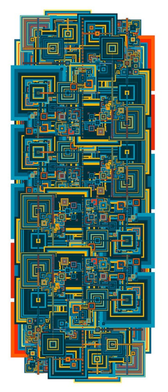
549
Figure 84. Algorithmic art: An artistic visual representation of multidimensional Hilbert
space (© Don Relyea).

550
Associated iterative C++ algorithm to create the artistic visual representation of a
multidimensional Hilbert space (i.e., infinite dimensional Euclidean space). The
algorithm is based on the Hilbert space filling curve:
227
on hilbert_draw(x0, y0, xis, xjs, yis, yjs, n)
–/* n=number of recursions*/
–/* numsteps= number of drawing iterations between two points on the
curve*/
–/* x0 and y0 are coordinates of bottom left corner */
–/* xis & xjs are the i & j components of unit x vector */
–/* similarly yis and yjs */
repeat while n > 0
hilbert_draw(x0, y0, yis/2, yjs/2, xis/2, xjs/2, n-1)
draw_from_to_numsteps( point(x0+xis/2, y0+xjs/2),
point(x0+(xis+yis)/2, y0+(xjs+yjs)/2), numsteps)
hilbert_draw(x0+xis/2, y0+xjs/2 ,xis/2, xjs/2, yis/2, yjs/2, n-1)
draw_from_to_numsteps( point(x0+xis/2, y0+xjs/2),
point(x0+(xis+yis)/2, y0+(xjs+yjs)/2), numsteps)
hilbert_draw(x0+xis/2+yis/2, y0+(xjs/2)+(yjs/2), xis/2, xjs/2,
yis/2, yjs/2,n-1)
draw_from_to_numsteps( point(x0+(xis/2)+(yis/2),
y0+(xjs/2)+(yjs/2)), point(x0+(xis+yis)/2, y0+(xjs+yjs)/2),
numsteps)
hilbert_draw(x0+(xis/2)+yis, y0+(xjs/2)+yjs, -yis/2,-yjs/2, -xis/2,
-xjs/2,n-1)
draw_from_to_numsteps( point(x0+xis/2+yis, y0+xjs/2+yjs),
point(x0+(xis+yis)/2, y0+(xjs+yjs)/2), numsteps)
n=n-1
227
See http://www.donrelyea.com/hilbert_algorithmic_art_menu.htm for further details.

551
if n=0 then exit repeat
end repeat
end
Code 2. Algorithmic digital art: C++ algorithm to create a visual representation of
multidimensional Hilbert space (© Don Relyea).

552
Psilocybin and the HT
2A
receptor
Psilocybin (O-phosphoryl-4-hydroxy-N,N-dimethyltryptamine) is an indole alkaloid
which is present in more than 150 fungi species, some of which are endemic to the UK.
Its molecular structure closely resembles serotonin (5-hydroxytryptamine, 5-HT). In
humans, psilocybin is rapidly dephosphorylated to psilocin (4-N,N-dimethyltryptamine)
which functions as a non-selective partial 5-HT receptor agonist and it shows
particularly high binding affinity for the 5-HT
1A
and 5-HT
2A
receptor subtypes (Carhart-
Harris & Nutt, 2017; Nichols, 2004). A landmark study conducted at Johns Hopkins
University by MacLean, Johnson & Griffiths (2011) experimentally demonstrated that a
single high-dose of psilocybin can induce long-lasting personality changes in the
domain “Openness to Experience”, as measured by the widely used NEO Personality
Inventory. Openness to Experience (OTE) is one of the core dimensions of the
extensively employed quinquepartite (big five) model of personality. OTE is an
amalgamation of several interconnected personality traits which include: 1) aesthetic
appreciation and sensitivity, 2) fantasy and imagination, 3) awareness of feelings in self
and others, and 5) intellectual engagement. Most relevant for the context at hand is the
fact that OTE has a strong and reliable correlation with creativity (Ivcevic & Brackett,
2015; S. B. Kaufman et al., 2016; Silvia et al., 2009)
228
. Individuals with high scores on
the OTE dimension are “permeable to new ideas and experiences” and “motivated to
enlarge their experience into novel territory” (DeYoung, Peterson, & Higgins, 2005).
228
For instance, the Pearson correlation coefficient for “global creativity” and OTE is .655 and for
“creative achievement” .481, By contrast, “Math–science creativity” is not statistically significantly
correlated with OTE (r =.059; ns; for further correlation between various facets of creativity and the Big
Five factors see Silvia, Nusbaum, Berg, Martin, & O’Connor, 2009). The salient correlation between
OTE and creativity has been reported in many studies (a pertinent meta-analysis has been conducted by
Feist, 1998; a recent study reporting a strong relationship between OTE and creativity has been conducted
by Puryear, Kettler, & Rinn, 2017). Furthermore, a meta-analytical structural equation model of 25
independent studies showed that OTE is the strongest FFM predictor of creative self-beliefs (r = .467;
Karwowski & Lebuda, 2016).
553
The experimentally induced increase in OTE was mediated by the intensity of the
mystical experience occasioned by psilocybin. Importantly, ego-dissolution is a central
feature of mystical experiences (see also Griffiths, Richards, McCann, & Jesse, 2006).
This finding is very intriguing because there is broad scientific consensus that
personality traits are relatively stable over time (i.e., a genetic basis is assumed;
Bouchard et al., 1990) and can only be altered by major life events (e.g., McCrae &
Costa, 1997). Hence, it has been experimentally demonstrated that psilocybin can have
profound influences on peoples deeply engrained thinking patterns, emotions, and
behaviours. For instance, psilocybin has been very successfully utilised for the
treatment of various addictions, major depression and anxiety disorders (for a review
see Bogenschutz & Ross, 2016).
Phenomenologically there is a significant degree of similarity between the qualitative
experiences induced by psilocybin and those reported by long-term meditators
(Griffiths, Richards, Johnson, McCann & Jesse, 2008). Interestingly, the neuronal
signature associated with psilocybin shows remarkable overlap with the neuronal
activity overserved during mediation (Brewer et al., 2011; cf. Carhart-Harris et al.,
2012), i.e., there is convergence between the phenomenology and the neural correlates.
Furthermore, mediation has been repeatedly associated with an altruistic orientation
(e.g., Wallmark, Safarzadeh, Daukantaitė & Maddux, 2012). A recent multimodal
neuroimaging study conducted by Tagliazucchi et al. (2016) conducted at Imperial
College London administered LSD intravenously to healthy volunteers. The researchers
found that LSD-induced ego-dissolution was statistically significantly correlated with
an increase in global functional connectivity density (FCD) between various brain
networks (as measured by fMRI). As discussed in the previous study by MacLean et al.
(2011), mystical experience is correlated with an increase in OTE which in turn is
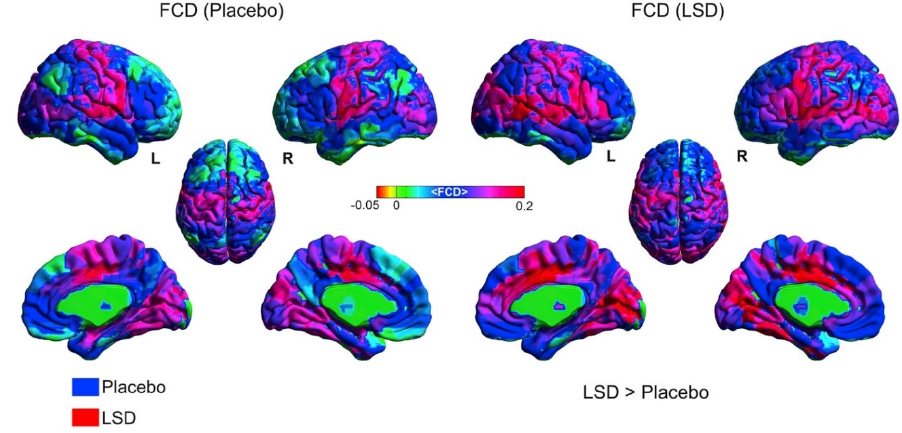
554
strongly correlated with creativity. One of the key findings of the current fMRI-study
was that high-level cortical regions and the thalamus displayed increased connectivity
under the acute influence of LSD. To be specific, increased global activity was observed
bilaterally in the high-level association cortices and the thalamus (often regarded as the
brains “central information hub” which relays information between various subcortical
areas and the cerebral cortices). The global activity increase in the higher-level areas
partially overlapped with the default-mode, salience, and frontoparietal attention
networks (see Figure 1). The FCD changes in the default-mode and salience network
were predicted a priori due their association with self-consciousness. As predicted, a
significant correlation between subjective ego-dissolution and activity changes in these
networks was detected. That is, the increase in global connectivity was significantly
correlated with self-report measures of ego-dissolution.
Figure 85. Average functional connectivity density Φ under the experimental vs. control
condition (adapted from Tagliazucchi et al., 2016, p. 1044)
The results demonstrate for the first time that LSD increases global inter-module
connectivity while at the same time decreasing the integrity of individual modules. The
observed changes in activity significantly correlated with the anatomical distribution of

555
5-HT
2A
receptors. Interestingly, LSD enhanced the connectivity between normally
separated brain networks (as quantified by the widely used Φ connectivity index
229
).
This result is especially relevant for researchers who want to identify the neural
correlates of creativity because an enhanced communication between previously
disconnected neuronal network modules is assumed to be crucial for the generation of
novel percepts and ideas (e.g., D. W. Moore et al., 2009). The authors concluded that
LSD reorganizes the rich-club architecture of brain networks and that this restructuring
is accompanied by a shift of the boundaries between self and environment. That is, the
ego-based dichotomy between self and other, subject and object, internal and external,
dissolves as a function of specific connectivity changes in the modular networks of the
brain
230
.
Taken together, Tagliazucchi et al. (2016) demonstrate that LSD induced ego-
dissolution is accompanied by significant changes in the neuronal rich-club architecture
and that ego-dissolution is accompanied by the downregulation of the default-mode
network (DMN). In the context of creativity research this finding is particularly
intriguing because the DMN is associated with habitual thought and behavior patterns
which are hypothesized to be negatively correlated with creativity and the generation of
novel ideas. That is, downregulation of the DMN by psychedelics and the
accompanying phenomenology of ego-dissolution are promising factors for the
229
The rich-club coefficient Φ is a networks metric which quantifies the degree to which well-connected
nodes (beyond a certain richness metric) also connect to each other. Hence, the rich-club coefficient can
be regarded as a notation which quantifies a certain type of associativity.
230
Furthermore, the authors argue convincingly that the notion that LSD (and other psychedelics)
“expand” consciousness is quantitatively supported by their data. Specifically, they argue that the
neurophysiological changes associated with psychedelic states contrast with states of diminished
consciousness (e.g., deep sleep or general anesthesia). The obtained results are congruent with the idea
that psychedelic and unconscious states can be conceptualized as polar-opposites on a continuous
spectrum of conscious states. Furthermore, the authors suggest that the level of consciousness is
quantitatively determined by the level of neuronal entropy (in accord with the entropic brain hypothesis
formulated by Carhart-Harris et al., 2014). It has been suggested that Aldous Huxley “reduction valve”
hypothesis appears to be relevant in this context.

556
understanding (and enhancement) of creativity.
231
Moreover, the cognitive flexibility
which appears to be associated with 5-HT
2A
agonism (see, for example, Carhart-Harris
& Nutt, 2017) is of particular relevance in the context of quantum cognition (and
quantum logic in general) because this counterintuitive framework requires a radical
reconceptualization (i.e., cognitive restructuring).
231
Recent evidence focusing on changes in the coupling of electrophysiological brain oscillations by
means of transfer entropy suggests that serotonergic psychedelics temporarily change information transfer
(via an increase of entropy?) within neural hierarchies by decreasing frontal of top-down control, thereby
releasing posterior bottom-up information transfer from inhibition (Francesc Alonso, Romero, Angel
Mañanas, & Riba, 2015).

557
Gustav Fechner on psychophysical
complementarity

558

559
“Man lives on earth not once, but three times: the first stage of his life is continual
sleep; the second, sleeping and waking by turns; the third, waking forever. In the first
stage man lives in the dark, alone; in the second, he lives associated with, yet
separated from, his fellow-men, in a light reflected from the surface of things; in the
third, his life, interwoven with the life of other spirits, is a higher life in the Highest of
spirits, with the power of looking to the bottom of finite things. In the first stage his
body develops itself from its germ, working out organs for the second; in the second
stage his mind develops itself from its germ, working out organs for the third ; in the
third the divine germ develops itself, which lies hidden in every human mind, to direct
him, through instinct, through feeling and believing, to the world beyond, which
seems so dark at present, but shall be light as day hereafter. The act of leaving the
first stage for the second we call Birth; that of leaving the second for the third, Death.
Our way from the second to the third is not darker than our way from the first to the
second: one way leads us forth to see the world outwardly; the other, to see it
inwardly.”
“On Life after Death” by Gustav Theodor Fechner (1801) translated from the German
by Hugo Wernekke.
URL: https://archive.org/stream/onlifeafterdeath00fech#page/30/mode/2up

560
Belief bias in syllogistic reasoning
An extensively phenomenon in the psychology of reasoning is termed belief bias (Evans
et al., 1983; Markovits & Nantel, 1989). Belief bias labels the long-standing effect that
reasoners are more likely to accept a believable conclusion to a syllogism
232
than an
unbelievable one, independent of the actual logical validity of the conclusion (i.e.
Wilkins, 1928; Henle & Michael, 1956; Kaufman & Goldstein, 1967). For instance,
examination of the following syllogism some basic definitions) shows that this
argument is logically invalid and that its conclusion does not concord with belief.
Consequently, endorsement rates are very low for this type of problem.
Major premise: No police dogs are vicious.
Minor premise: Some highly trained dogs are vicious.
Conclusion: Some police dogs are not highly trained.
232
A categorical syllogism (Greek: συλλογισμός svullogisvmìc - conclusion or inference) consists of three parts: the
major premise, the minor premise and the conclusion, for example:
Major premise: All animals are mortal.
Minor premise: All humans are animals.
Conclusion: Ergo, all humans are mortal.
Or in Aristotle’s terms: “Whenever three terms are so related to one another that the last is contained in the middle as
in a
whole, and the middle is either contained in, or excluded from, the first as in or from the whole, the extremes must be
related by a perfect syllogism. I call that term ‘middle‘ which is itself contained in another and contains another in
itself.”
(Aristotle, Prior Analytics 25b, as cited in Lakoff & Johnson, 1999)

561
Interestingly, one can construct syllogisms in which validity and believability are
discordant, as in the following argument:
Major premise: No addictive things are inexpensive.
Minor premise: Some cigarettes are inexpensive.
Conclusion: Some addictive things are not cigarettes.
In this example the syllogism is invalid, but the conclusion is believable. Upon
inspection, it can be determined that the two exemplary syllogisms have the same
logical form. Despite this fact, a major proportion of participants judge the fallacious
but believable conclusion as valid, that is, participants exhibit the tendency to judge the
validity of a syllogism based on its a priori believability. In their research Evans et al.
(1983) reported two main effects, first, participants affirm more believable than
unbelievable conclusions and, second, more logically valid than invalid conclusions.
Moreover, there was a significant interaction between believability and validity. The
effects of belief are stronger on logically invalid than on valid syllogisms. This
phenomenon is one of the most prevalent content effects studied in deductive reasoning
(for a comprehensive review see Klauer et al., 2000) and it has been demonstrated that
response bias to a given syllogism can be influenced by several factors, for example,
perceived difficulty of the syllogism (Evans, 2009a), caution (Pollard & Evans, 1980),
atmosphere bias (Begg & Denny, 1969), figural bias (Dickstein, 1978; Morley et al.,
2004; Jia et al., 2009), presentation order (Lambell et al., 1999), and perceived base rate
of valid syllogisms (Klauer et al., 2000), to name just the most prominent factors.
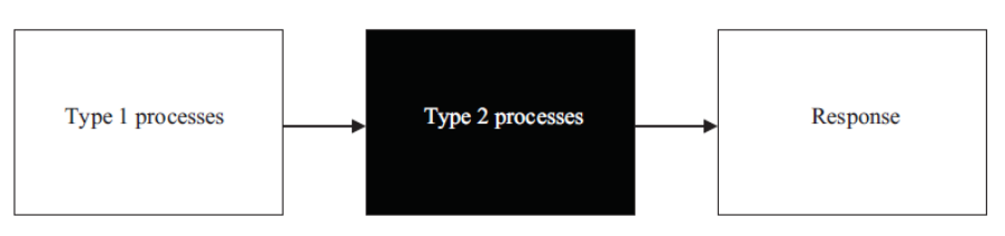
562
A widely acknowledged descriptive explanation for the belief bias effect is termed the
default interventionist (DI) account (see Evans, 2007). Following this account Type 1
and Type 2 processes succeed one another in a sequential order. Primacy is attributed to
Type 1 (heuristic) processes which generate a default response whereas recency is
ascribed to Type 2 (analytic) processes which approve or override the response
generated by Type 1 processes (Stanovich & West, 2000; De Neys, 2006; Evans, 2007;
Stanovich, 2008). The process of computing the correct solution and overriding the
response cued by Type 1 processes is assumed to be costly in cognitive terms, drawing
on limited executive resources. The DI process model is visualized in Figure 86.
Figure 86. Flowchart depicting the default-interventionist model.
In support of this account, Evans & Curtis-Holmes (2005) showed that rapid responding
increases belief bias in a deductive reasoning task. Conceptually related studies
indicated that participants with high working memory spans performed better on a
reasoning task than those with lower spans when believability of a conclusion conflicted
with its logical validity (De Neys, 2006) and that the inhibition of initial responses is
related to the capacity of inhibitory processes which covaries with age (De Neys &
Franssens, 2009). Further quasi-experimental studies suggest that ecstasy users, due to
their reduced working memory capacity, perform worse on syllogistic reasoning tasks
than nonusers (Fisk et al., 2005). Other variables that have been related to analytic
thinking are, for example, actively open-minded thinking and need for cognition (Kokis

563
et al., 2002). Moreover, recent research suggests that cognitive load has detrimental
effects on logical reasoning performance (De Neys, 2006; De Neys & Van Gelder,
2009). In addition, experimental findings summarized by Stanowich (1999) suggest that
belief-bias is negatively related to cognitive capacity, that is, individuals low in
cognitive capacity are more likely to respond on the basis of belief as compared to logic.
It should be empathized that the limited capacity of Type 2 processes is a common
theme in much of the cited work. In the context of quantum cognition, it should be
emphasised that the empirical scientific facts associated with quantum theory stand in
sharp contrast with our prior beliefs about logic and reality in general. Therefore, belief-
bias is of great pertinence for the context at hand because it can be predicted that beliefs
negatively interfere with logic-based rational argument evaluation (i.e., prior belief bias
the logical conclusion in a n irrational manner). Other cognitive biases which are
relevant in this respect are confirmation bias (M. Jones & Sugden, 2001; Nickerson,
1998; Oswald & Grosjean, 2004; Rajsic et al., 2015) and asymmetric Bayesian belief
updating
233
(Loewenstein & Lerner, 2003; Moutsiana, Charpentier, Garrett, Cohen, &
Sharot, 2015; Moutsiana et al., 2013). Both biases account for the human propensity to
maintain false beliefs in the face of contradicting evidence. However, a detailed
discussion goes beyond the scope of this thesis and we refer the interested reader to the
cited literature for further information.
233
Asymmetric belief updating has also been termed “valence-dependent belief updating” as it refers to
“greater belief updating in response to favourable information and reduced belief updating in response to
unfavourable information” (Moutsiana et al., 2015, p. 14077)

564
Dual-process theories of cognition
Dual-process theories in cognitive psychology hypothesize two qualitatively discernible
cognitive processes that operate according to fundamentally different principles.
Second-generation cognitive scientists use terms like automatic vs. controlled
(Kahneman, 2003), heuristic vs. analytic (Klaczynski, 2001a, 2001b), intuitive vs.
reflective (Sperber, 1997), associative vs. rule based (Sloman, 1996), personal vs.
subpersonal (Frankish & Evans, 2009), analogue vs. symbolic (Paivio, 1986), reflexive
vs. reflective (Lieberman et al., 2002), et cetera. In social psychology dual-process
theorists also use a multifarious nomenclature. For instance, heuristic vs. systematic
(Chaiken, 1980), peripheral vs. central (Petty & Cacioppo, 1981, 1984), implicit vs.
explicit (Greenwald et al., 1998), automatic vs. conscious (Baumeister, 2005),
experiential vs. noetic (Strack & Deutsch, 2004), associative vs. propositional
(Gawronski & Bodenhausen, 2006), to name just the most popular terms. However, it
has been noted that “what matters is not the specific names but the fact of duality”
(Baumeister, 2005, p.75). There is remarkable resemblance between dual process
models conglomerated in social psychology and those accrued in cognitive psychology.
Evans (2009a) criticizes that there have been few attempts to integrate dual-process
theories across the different psychological paradigms (for exceptions see E. R. Smith &
DeCoster, 2000 or (Barrett et al., 2004)). The now widely used umbrella terms System 1
and System 2 which are used to label the two postulated processes were first introduced
by Stanowich (1999). A comprehensive summary of the features attributed to each
system has been compiled by Frankish (2009) and is reprinted (in adapted form) in
Table 39.

565
Table 39
Features attributed by various theorists to the hypothesized cognitive systems.
System 1
System 2
Evolutionarily old
Shared with animals
Implicit
Automatic
Parallel
Fast
High capacity
Intuitive
Unconscious
Contextualized
Semantic
Associative
Not linked to general intelligence
Independent of executive functions
Evolutionarily recent
Uniquely human
Explicit
Controlled
Sequential
Slow
Low capacity
Reflective
Conscious
Abstract
Logical
Rule-based
Linked to general intelligence
Dependent on executive functions
Nobel Prize winner Daniel Kahneman is momentarily presumably the most famous dual
process theory proponent. During his Nobel Prize lecture
234
he introduced his research
project as an “attempt to map departures from rational models and the mechanisms that
explain them”. Moreover, one of the main points on his agenda was to “introduce a
general hypothesis about intuitive thinking, which accounts for many systematic biases
that have been observed in human beliefs and decisions” (Kahneman, 2002). He
234
Associated URL of the official Nobel Prize lecture (2002, Stockholm University):
https://www.nobelprize.org/mediaplayer/index.php?id=531
566
advocates an evolutionary perspective on reasoning and his reflections are based on the
assumption that there is a kind of quasi biogenetic progression in the evolution of
cognitive processes starting from automatic processes which form the fundamental basis
for the evolution of more deliberate modes of information processing. The
“phylogenetic” history of higher order cognitive processes could be adumbrated as
follows:
PERCEPTION → INTUITION → REASONING
According to this view, perception appears early on the timeline of evolutionary history
whereas reasoning evolved relatively recently. Intuition is intermediate between the
automatic processes of perception and the deliberate, higher order reasoning processes
that are the hallmark of human intelligence (Kahneman, 2003). Furthermore, he
proposes that intuition is in many ways similar to perception and the analogy between
perception and intuition is the common denominator of much of his work. Perception is
a highly selective process which focuses on certain characteristics of the environment
neglecting others. One could argue that reality is a continuous multimodal attack on our
senses. The perceptual system deals with this in different ways. For example, we
perceive discrete events (Tversky et al., 2008) and exclude irrelevant features from
perception (Lavie et al., 2004; Simons & Chabris, 1999) whereas other features “pop-
out” due to their salience (Treisman & Gelade, 1980). Moreover, some features are
directly available to perception whereas other features are not. Kahneman argues that
most of the time we do not engage in effortful thinking and reasoning. Our standard
mode of operations is intuitive thinking. This is the fundamental assumption underlying
the two-system view, which differentiates between intuition and reasoning. In the
context of dual process theories of reasoning Kahneman (2003) argues that System 1
processes are responsible for repeating simple and automatic operations, whereas
567
System 2 processes are accountable for deliberate mental operations and the detection
and correction of errors made by System 1. In order to illustrate the dual-system
approach we would like the reader to answer the following question (adapted from
Frederick, 2005):
A BAG AND A BOOK COST TOGETHER £110.
THE BAG COST £100 MORE THAN THE BOOK.
WHAT DOES THE BOOK COST?
For most people the first thing that comes to mind is £10. Of course, this answer is
incorrect. Using the terminology of dual-process theories, System 1 has produced a fast
heuristic response and the slower System 2 is able to scrutinize this response
analytically and might eventually correct it. This example neatly demonstrates the
heuristic vs. analytic distinction in dual-process theory (Evans, 2006; Kahneman, 2003;
Klaczynski, 2001b). Sloman (2002) also supports the notion of two different systems of
reasoning and proclaims that people can believe in two contradictory responses
simultaneously. Sloman articulates that “the systems have different goals and are
specialists at different kinds of problems” (Sloman, 1996, p.6). In order to elucidate his
argumentative line he uses an example of a judge (Sloman, 2002). Judges often have to
neglect their personal beliefs and decide a given case on the basis of evidence according
to the law. It is thus possible that the belief-based response of the judge continues to be
compelling regardless of certainty in the second response based on the juridical law. In
addition, Sloman (2002) employs the classical Müller-Lyer illusion (Müller-Lyer, 1889)
in order to illustrate that two independent systems are at work (see Figure 87).
568
Figure 87. The Müller-Lyer illusion (Müller-Lyer, 1889).
Even when the percipient knows that the two lines are of equal length the two lines are
still perceived as different. In other words, explicit knowledge (System 2) about
physical reality does not alter the visual percept (System 1). This classical example
provides anecdotal evidence for the existence of two cognitive systems, because people
can believe in two contrary responses simultaneously. A rich body of research
demonstrates that the balance between these two stipulated types of thinking can be
shifted. Methods for shifting the balance to System 1 processes involve concurrent
working memory load (Gilbert, 1991) in order to interfere with System 2 processes and
the use of time pressure (Finucane et al., 2000) to impose temporal processing
constrains on System 2. Moreover, System 2 processing can be facilitated by explicitly
instructing people to employ logical reasoning (Klauer et al., 2000). In addition, there
are dispositional factors which are correlated with the functioning of System 2, for
instance, individual differences variables like the extensively studied “need for
cognition” (Shafir & LeBoeuf, 2002) and general cognitive ability (Stanovich & West,
1998, 2000). In addition, individual differences in executive functioning, working-
memory capacity, and self-control appear to play a pivotal role in this context. From a
neuroscientific point of view, the prefrontal cortices (PFC) are assumed to be
569
responsible for executive control of different tasks (Miller & Cohen, 2001). However,
precise localization of function is difficult because the brain is a complex and integrated
system. Many researchers argue against a fully modular and departmentalized
anatomical view and for a continuous view on psychological constructs and processes
(but see Stuss, 1992). It has been noted that, “it is entirely possible that, although the
frontal lobes are often involved in many executive processes, other parts of the brain
may also be involved in executive control” (Baddeley, 1996, p. 6-7; see also Braver et
al., 1997). However, it seems as if certain brain regions are more involved in executive
functioning than others and the prefrontal cortices have been associated with executive
control function (Della Sala et al., 1998), supervisory system (Shallice, 2001; Alexander
et al., 2007), and dysexecutive syndrome (Baddeley & Wilson, 1988; Laine et al.,
2009). Three regions seem to be particularly involved in executive functioning, working
memory, and self-control: 1) the dorsolateral prefrontal cortex (DL-PFC) 2) the
ventromedial prefrontal cortex (vmPFC) and 3) the and the anterior cingulate cortex
(ACC) (see Figure 88).
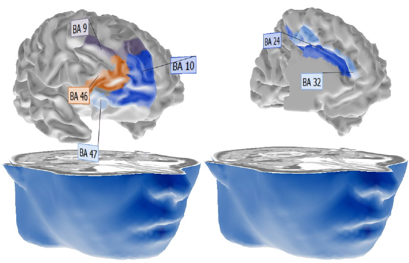
570
Figure 88. Neuroanatomical correlates of executive functions (DL-PFC, vmPFC, and
ACC)
Left picture: Dorsolateral prefrontal cortex (Brodmann area 46 and 9), ventromedial
prefrontal cortex (BA10) and inferior prefrontal gyrus (BA47). Right picture: ventral
(BA24) and dorsal (BA32) anterior cingulate cortex. 3D graphics were created using the
“BrainVoyager” software package (Goebel, 2007).
Space does not permit a detailed discussion of these neuroanatomical structures which
appear to be crucial for sound logical reasoning and the inhibition of
(habitual/automatic) belief-based responses. However, we will briefly outline some of
the main characteristics in the following paragraphs (we refer the interested reader to
Miller & Cohen, 2001). For instance, Fuster (1997) argued that the DL-PFC houses
working memory whereas the ventral-prefrontal cortex is associated with inhibition of
(automatic) behavioural responses. However, other researchers (e.g., May et al., 1999)
571
disagreed, claiming that this functional dichotomy is not evident because the processes
are concatenated and dependent on one another. It has been suggested that the
dorsolateral prefrontal cortex is associated with the implementation of cognitive control,
executive functioning, working memory, attentional switching and selective attention,
whereas the ventromedial prefrontal cortex is assumed to moderate amygdala activity,
that is, emotions and emotional reactions (Bechara et al., 1999; Duncan & Owen, 2000).
The anterior cingulate cortex is assumed to be involved in performance monitoring and
detection of conflict and selection of appropriate responses (MacDonald et al., 2000;
Miller & Cohen, 2001; Pochon et al., 2008; Posner & Rothbart, 2009). Based on
imaging data and lesion studies researchers concluded that especially the dorsal ACC is
very likely involved in situations that involve decision making, conflict, and inhibition
(Ochsner & Gross, 2004, p.236). Moreover, it has been suggested that self-control and
executive functions are both associated with an increase in anterior cingulate cortex
activity (but see Posner et al., 2007).

572
Bistability as a visual metaphor for paradigm
shifts
Figure 89. Bistable visual stimulus used by Thomas Kuhn in order to illustrate the
concept of a paradigm-shift.
Thomas Kuhn used the duck-rabbit (Brugger, 1999) to illustrate the fundamental
perceptual change that accompanies a scientific paradigm-shift. The concept of
incommensurability is pertinent in this context, i.e., the impossibility of direct
comparison of complementary theories. It is impossible to see both percepts
simultaneously (it is either a rabbit or a duck – the ambiguous superposition of both
cannot be perceived by the visual system). In the same way, it is impossible to entertain
conflicting scientific paradigms simultaneously. The human cognitive system
automatically reduces ambiguity and thrives for closure (Webster & Kruglanski, 1994).
In contemporary psychology, bistable perception is a topic of ongoing research (Sterzer
& Rees, 2010). Recently, it has been investigated in the theoretical framework of

573
quantum cognition, i.e., with respect to the complementarity principle and the quantum-
zeno effect (Atmanspacher & Filk, 2010, 2013, Atmanspacher et al., 2004, 2009).
Harald Atmanpachers’ creative idea was to treat the underpinning process of bistable
perception in terms of the evolution of an unstable two-state quantum system. In
quantum physics, the quantum Zeno effect is a situation in which an unstable particle, if
observed continuously, will never decay. To be precise, “The coupling of an unstable
quantum system with a measuring apparatus alters the dynamical properties of the
former, in particular, its decay law. The decay is usually slowed down and can even be
completely halted by a very tight monitoring.” (Asher Peres, 1980)
The Zeno effect is also known as the Touring paradox:
“It is easy to show using standard theory that if a system starts in an eigenstate of some
observable, and measurements are made of that observable N times a second, then,
even if the state is not a stationary one, the probability that the system will be in the
same state after, say, one second, tends to one as N tends to infinity; that is, that
continual observations will prevent motion …”
— Alan Turing as quoted by A. Hodges in Alan Turing: Life and Legacy of a Great
Thinker p. 54
CogNovo NHST survey: A brief synopsis
“Few researchers are aware that their own heroes rejected what they practice routinely.
Awareness of the origins of the ritual and of its rejection could cause a virulent cognitive
dissonance, in addition to dissonance with editors, reviewers, and dear colleagues. Suppression
of conflicts and contradicting information is in the very nature of this social ritual.” (G
Gigerenzer, 2004, p. 592)
574
Null hypothesis significance testing (NHST) is one of the most widely used inferential statistical
techniques used in science. However, the conditional syllogistic logic which underlies NHST is
often poorly understood by researchers. That is, researchers using NHST often misinterpret the
results of their statistical analyses. Fallacious scientific reasoning is a problem with huge
ramifications. If researchers regularly misinterpret the meaning of p-values this implies that the
conclusions, they derive from their research are often logically invalid. How often is an
empirical question which is worth investigating in more detail.
This paper briefly describes the results of a small-scale survey we conducted at the
interdisciplinary “CogNovo Research Methods Workshop” at Plymouth University in June
2014. Participants were Phd students, research fellows, lecturers, and professors who attended
the workshop with the adequate title “The Pitfalls of Hypothesis Testing”. At the very beginning
attendees were asked to interpret the results of the following simple independent means t test.
Participants were asked to mark each of the statements below as “True” or “False” (adapted
from Oakes, 1986).
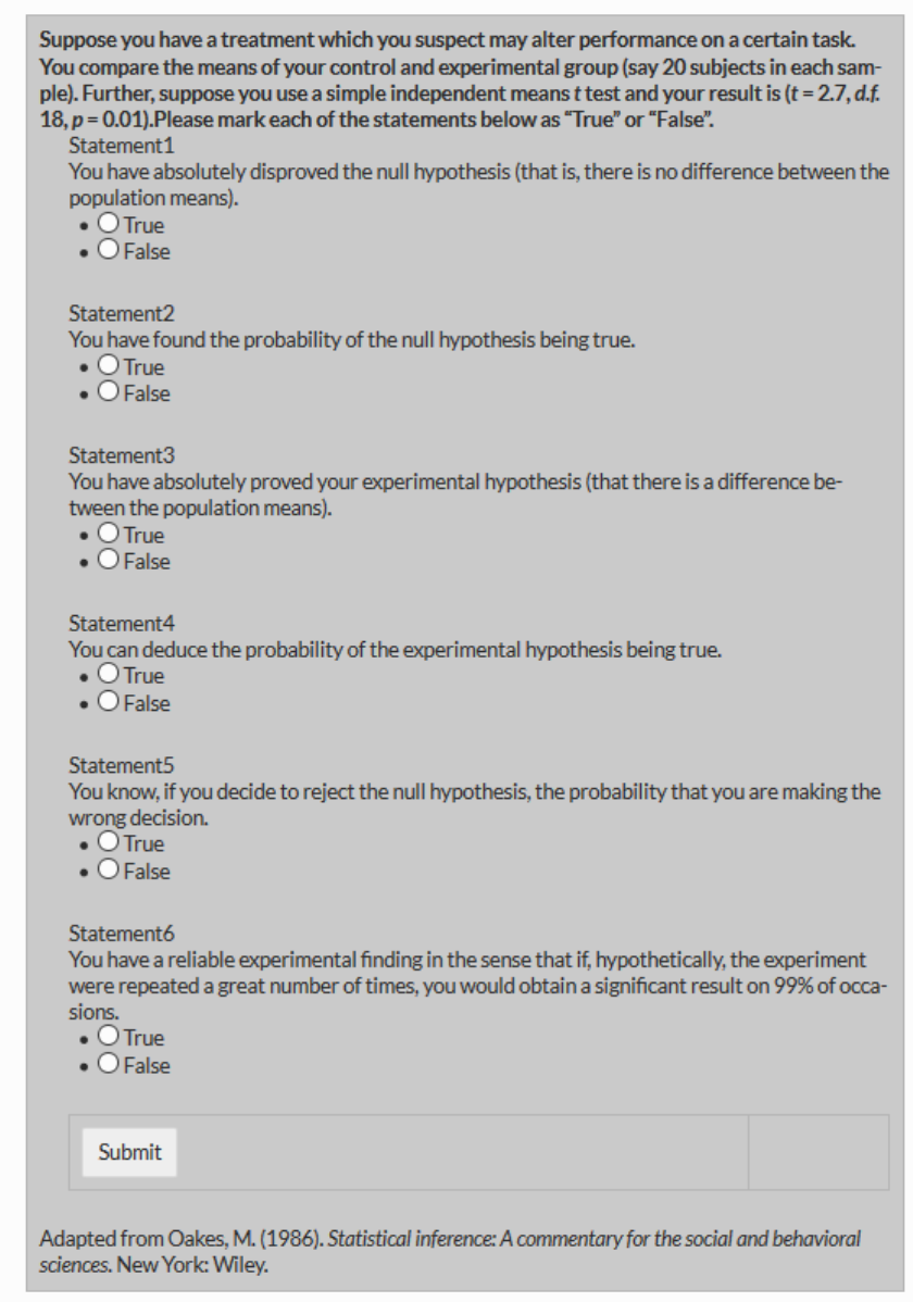
575

576
The t test at hand is a very basic exemplar of the kind of significance testing which many
scientists routinely employ. Hence, its correct interpretation is of paramount importance for
many far-reaching real-world decisions and the progress of science in general.
In our experiment we utilized a custom-made web-based questionnaire in order to collect the
responses from participants. The HTML code utilised responsive web-design CSS -techniques
which allowed participants to visit the website immediately (during the lecture) on various
devices with varying resolution (laptops, tablets, smart-phones, ect.). We asked only those
workshop attendees who had prior experience with statistical significance testing to participate.
A total of 18 participants responded to each of the 6 statements within ≈ 5minutes by using their
mobile phones, notebooks, or tablets. The resulting data-set is available under the following
URL:
https://docs.google.com/spreadsheets/d/1qEcJGoCBMDCXNbkttgZirWJzNJRqyxFEmHzk8hT
oZhk/edit?usp=drive_web#gid=0
The lecture itself is available on YouTube under the following URL:
https://youtu.be/wOYgQzCLiBQ?t=1939
The powerpoint slides used in this presentation can be downloaded as a PDF.
http://irrational-decisions.com/hypothesis-testing%20-full-web-version.pdf
(password: cognovo)
We analysed the data in real-time during the presentation of the talk using the following
custom-made R code which utilises the RCurl package (Lang, 2006) to pull the data from the
server.
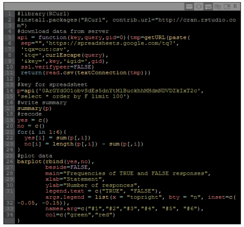
577
Altogether, only one participant responded correctly to all statements. The remaining 17
participants indicated that at least 1 of the 6 statements would be correct. Note that the p-value
is the probability of the observed data (or of more extreme data points), given that the null
hypothesis H
0
is true, defined in symbols as p(D|H
0
). The results of the survey are visualized in
Figure 1.
Logical fallacies in interpretation
The following paragraphs will deconstruct the logical fallacies committed by the majority of
participants (see Cohen, 1994, 1995, G Gigerenzer, 1993, 1998, 2004).
Statements 1 and 3 are easily detected as logically invalid. A significance test can never prove
or disprove the null hypothesis or the experimental hypothesis with certainty. Statement 1 and 3
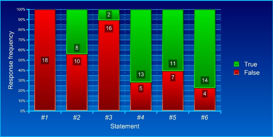
578
are instances of the epistemological illusion of certainty (G Gigerenzer & Krauss, 2004). As can
be seen in Figure 1, all participants gave the correct response to statement 1, however, 2
participants believed that statement 2 is true.
Statements 2 and 4 are also false. The probability p(D|H
0
) is not the same as p(H
0
|D), and more
generally, a significance test does never provide a probability for a hypothesis. To equate the
direct probability with its inverse is an illusionary quasi-Bayesian interpretation of p(D|H
0
). This
has been termed the inverse problem.
Figure 90. Results of CogNovo NHST survey
Equation 13. The inverse probability problem
p(D|H
0
) ≠ p(H
0
|D)
This particular illusion has been perpetuated by many statistics textbooks (for further examples
see Gigerenzer, 2000). For instance, in one of the early texts “Guilfords’ Fundamental Statistics
in Psychology and Education” the p values turns miraculously into a Bayesian posterior
probability:
579
“If the result comes out one way, the hypothesis is probably correct, if it comes out another
way, the hypothesis is probably wrong” (p. 156). Guilford is no exception. He signifies the
beginning of a class of statistical texts that presents significance testing as a hybrid between
Fisherian and Neyman/Pearsonian methods without mentioning its origins (Gigerenzer 2000
terms this “the denial of parents”). Neither Fisher or Neyman/Pearson would have agreed upon
the hybrid method because they disagreed vehemently. The currently used hybrid additionally
confuses the researchers’ desire for probabilities of hypotheses and what significance testing can
actually provide (that is, a Baysian interpretation is added to the already incompatible
combination).
Statement 5 also refers to a probability of a hypothesis. This is because if one rejects the null
hypothesis, the only possibility of making a wrong decision is if the null hypothesis is true.
Thus, it makes essentially the same claim as Statement 2 and 4 do, and both are incorrect.
Statement 6 amounts to the replication fallacy (Gigerenzer, 1993, 2000). Here, p=1% is taken
to imply that such significant data would reappear in 99% of the repetitions.
However: p(D|H
0
) does not entail any information about p(replication)
Especially the replication fallacy seems to be widespread. For example, the editor of the top-
ranking Journal of Experimental Psychology stated that he used the level of statistical
significance reported in submitted papers as the measure of the “confidence that the results of
the experiment would be repeatable under the conditions described” (Melton, 1962, p. 553).
Contrary to his belief, the p-value conveys no information at all about the replicability of an
experimental finding.
Logical inconsistency between responses
Statement 2, 4, and 5 are logical implications of one another. To be logically consistent all three
statements should either be rejected or approved.
• 8 participants were inconsistent when responding to statement 2, 4, and 5.
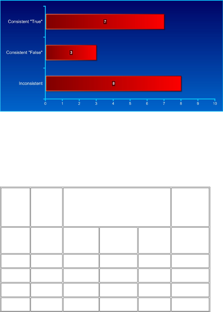
580
• 3 participants described all three statements correctly as false.
• 7 (although wrongly) described all three statements as true.
Figure 91. Logical consistency rates
International comparison with other universities
Table 40.
Comparison between international universities and between academic groups.
Plymouth
University
(UK)
Psychological Departments
German Universities
USA
(Oakes, 1986)
Current
experiment
Methodology
Instructors
Scientific
Psychologists
Psychology
Students
Academic
Psychologists
#1)
0%
10%
15%
34%
1%
#2)
44%
17%
26%
32%
36%
#3)
11%
10%
13%
20%
6%
#4)
61%
33%
33%
59%
66%

581
#5)
72%
73%
67%
68%
86%
#6)
77%
37%
49%
41%
60%
Overall, statement 1, 2, and 3 are more often correctly falsified as compared to statement 4, 5,
and 6.
Table 41
Fallacious NHST endorsement rates per group.
Professors and lecturers teaching statistics
(N=30):
80%
Professors and lecturers
(N=39):
90%
Students
(N=44):
100%
Table 2. The amount of wrong interpretations of p = 0.01. The table shows the
percentage in each group who endorsed one or more of the six false statements (Haller
& Krauss, 2002).
Brief discussion
The results of this investigation have serious implications because they demonstrate that the
misinterpretation of NHST is still a ubiquitous phenomenon among researchers in different
fields, despite the fact that this issue has been strenuously pointed out repeatedly before
(Rozeboom , 1960; Meehl, 1978; Loftus, 1991; Simon, 1992; Gigerenezer, 1993; Cohen, 1994).
We argue that wishful Bayesian thinking (made possible by fallaciously mistaking direct
582
probabilities for inverse probabilities) lies at the core of these pertinacious cognitive illusions.
Unfortunately, far reaching real world decisions are based on the conclusions drawn from these
demonstrably widely misunderstood test procedures.Therefore, educational curricula should
make sure that students understand the logic of null hypothesis significance testing.
The syllogistic logic of NHST
From a logical point of view NHST is based upon the logic of conditional syllogistic reasoning
(Cohen, 1994). Compare the following syllogisms of the form modus ponens:
Syllogism 1
1
st
Premise:
If the null hypothesis is true, then this data (D) can not occur.
2
nd
Premise:
D has occurred.
Conclusion:
H
0
is false.
If this were the kind of reasoning used in NHST then it would be logically correct. In the
Aristotelian sense, the conclusion is logically valid because it is based on deductive proof (in
this case denying the antecedent by denying the consequent). However, this is not the logic
behind NHST. By contrast, NHST uses hypothetical syllogistic reasoning (based on
probabilisties), as follows:
Syllogism 2
1
st
Premise:
If H
0
is true, then this data (D) is highly unlikely.
2
nd
Premise:
D has occurred.
583
Conclusion:
H
0
is highly unlikely.
By making the major premise probabilistic (as oposed to absolute, cf. Syllogism 1) the
syllogism becomes formally incorect and consequently leads to an invalid conclusion. The
following structure of syllogistic reasoning is implicitly used by many authors in uncountable
published scientific articles. This logical fallacy has been termed the “the illusion of attaining
improbability”. (Cohen, 1994, p.998).
Syllogism 3
1
st
Premise:
If H
0
is true, then this data (D) is highly unlikely.
2
nd
Premise: D
has occurred.
Conclusion:
H
0
is probably false.
Note: p(D|H
0
) ≠ p(H
0
|D)
Belief bias and wishful thinking in scientific reasoning
Most importantly, all fallacious interpretations are unidirectional biased: they make the
informational value of p appear bigger than it in reality is. In other words, researchers are
positively biased with regards to the interpretation of p-values because they attribute more
informational value to the p-value than it actually contains.
Cohen (1994, p.997) formulated the problem very clearly: “What’s wrong with significance
testing? Well, among many other things, it does not tell us what we want to know, and we so
much want to know what we want to know that, out of desperation, we nevertheless believe in
that it does! What we want to know is ‘given these data, what is the probability that H
0
is true?

584
But as most of us know, what it tells us is given that H
0
is true, what is the probability of these
or more extreme data.” (italics added)
Moreover, Gigerenzer (2000) clearly agrees with Cohen (1984) that the currently used hybrid
logic of significance testing is “A mishmash of Fisher and Neyman-Pearson, with invalid
Bayesian interpretation” (Cohen, 1994, p. 998). The historical genesis of the hybrid is very
revealing. An eye-opening historical perspective on the widely unacknowledged but fierce
debate between Fisher and Neyman/Pearson is provided by Gigerenzer (1987).
Broader implications
Given that inferential statistics are at the very heart of scientific reasoning it is essential that
researchers have a firm understanding of the actual informative value which can be derived
from the inferential techniques they employ in order to be able to draw valid conclusions.
Future studies with academicians and PhD students from different disciplines are needed to
determine the epidemiology
235
of these statistical illusions. The next step would be to develop
and study possible interventions (but see Lecoutre et al., 2003).
We suggest that is necessary to development novel pedagogical concepts and curricula in order
to teach the logic of NHST to students. Moreover alternative statistical inferential methods
should be taught to students given that there is no “magic bullet” or “best” inferential method
per se. Gigerenzer (1993) points out that “it is our duty to inform our students about the many
good roads to statistical inference that exist, and to teach them how to use informed judgment to
decide which one to follow for a particular problem” (p. 335). We strongly agree with this
proposition.
Pertinent citations from eminent psychologists
235
Epidemiology literally means “the study of what is upon the people”and the term is derived from
Greek epi, meaning “upon, among”, demos, meaning “people, district”, and logos, meaning “study, word,
discourse”. In that sense, the current investigation can be regarded as an ethnographgic studie.
585
“I suggest to you that Sir Ronald has befuddled us, mesmerized us, and led us down the
primrose path. I believe that the almost universal reliance on merely refuting the null
hypothesis is one of the worst things that ever happened in the history of psychology.”
(Meehl, 1978, p. 817; Former President of the American Psychological Association, inter
alia)
The eminent and highly influential statistician Jacob Cohen argues that null hypothesis
significance testing „not only fails to support the advance of psychology as a science but
also has seriously impeded it.“ (Cohen, 1997, p. 997; * 1923; † 1998; Fellow of the
American Association for the Advancement of Science, inter alia)
“Few researchers are aware that their own heroes rejected what they practice routinely.
Awareness of the origins of the ritual and of its rejection could cause a virulent cognitive
dissonance, in addition to dissonance with editors, reviewers, and dear colleagues.
Suppression of conflicts and contradicting information is in the very nature of this social
ritual.” (Gigerenzer, 2004, p. 592; Director Emeritus of the Center for Adaptive Behavior
and Cognition at the Max Planck Institute for Human Development, inter alia)
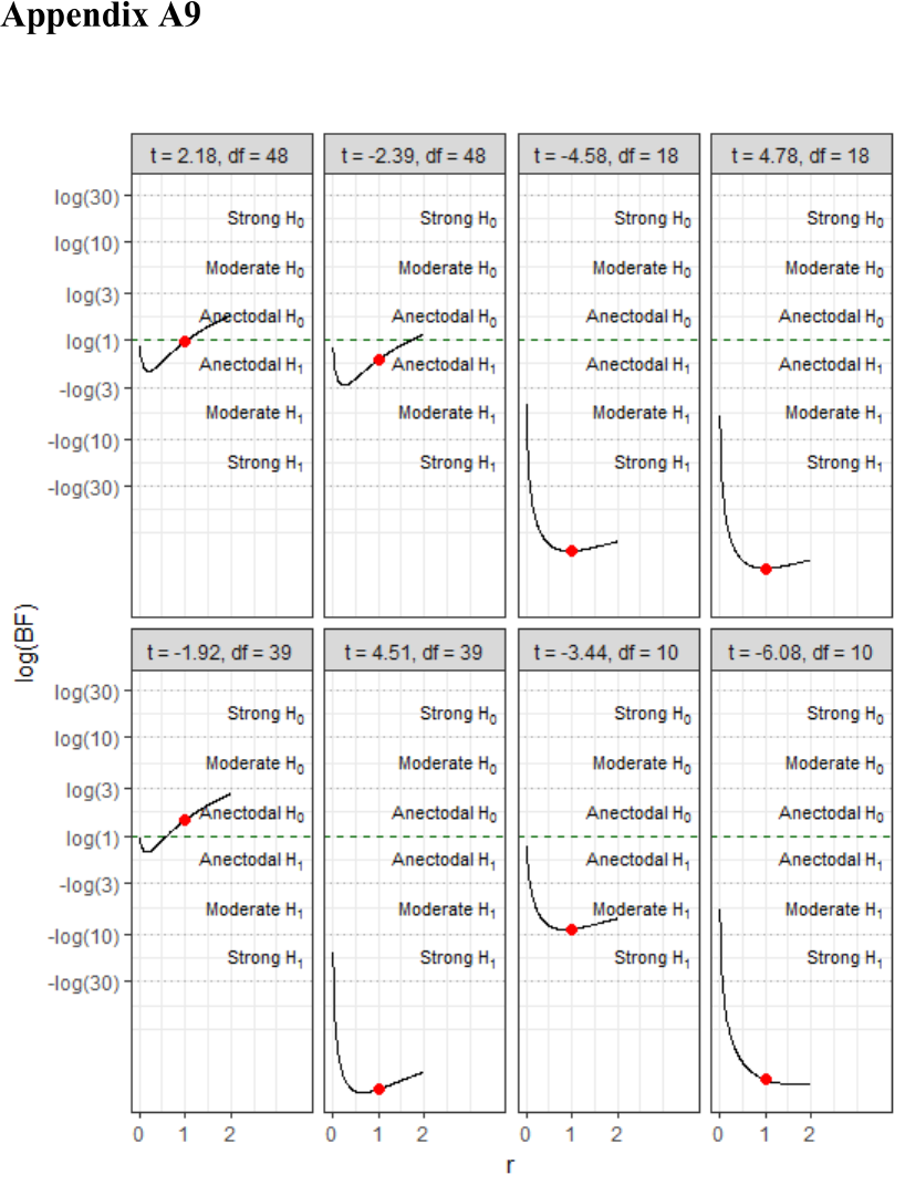
586
Reanalysis of the NHST results reported by
White et al. (2014) in a Bayesian framework
Figure 92. Bayesian reanalysis of the results NHST reported by White et al., 2014.

587
Note that the results are not entirely congruent the with conclusions drawn from the
NHST analysis. The associated R code which utilises the “BayesFactor” package (R
D. Morey & Rouder, 2015) is appended below.
## This source code is licensed under the FreeBSD license
## (c) 2013 Felix Schönbrodt
# Morey, R. D., Rouder, J. N., & Jamil, T. (2014). BayesFactor: Computation
of Bayes factors for common designs. R Package Version 0.9, 8.
install.packages("BayesFactor")
#' @title Plots a comparison of a sequence of priors for t test Bayes
factors
#'
#' @details
#'
#'
#' @param ts A vector of t values
#' @param ns A vector of corresponding sample sizes
#' @param rs The sequence of rs that should be tested. r should run up to 2
(higher values are implausible; E.-J. Wagenmakers, personal communication,
Aug 22, 2013)
#' @param labels Names for the studies (displayed in the facet headings)
#' @param dots Values of r's which should be marked with a red dot
#' @param plot If TRUE, a ggplot is returned. If false, a data frame with
the computed Bayes factors is returned
#' @param sides If set to "two" (default), a two-sided Bayes factor is
computed. If set to "one", a one-sided Bayes factor is computed. In this
case, it is assumed that positive t values correspond to results in the
predicted direction and negative t values to results in the unpredicted
direction. For details, see Wagenmakers, E. J., & Morey, R. D. (2013).
Simple relation between one-sided and two-sided Bayesian point-null
hypothesis tests.
#' @param nrow Number of rows of the faceted plot.
#' @param forH1 Defines the direction of the BF. If forH1 is TRUE, BF > 1
speak in favor of H1 (i.e., the quotient is defined as H1/H0). If forH1 is
FALSE, it's the reverse direction.
#'
#' @references
#'
#' Rouder, J. N., Speckman, P. L., Sun, D., Morey, R. D., & Iverson, G.
(2009). Bayesian t-tests for accepting and rejecting the null hypothesis.
Psychonomic Bulletin and Review, 16, 225-237.
#' Wagenmakers, E.-J., & Morey, R. D. (2013). Simple relation between one-
sided and two-sided Bayesian point-null hypothesis tests. Manuscript
submitted for publication
#' Wagenmakers, E.-J., Wetzels, R., Borsboom, D., Kievit, R. & van der
Maas, H. L. J. (2011). Yes, psychologists must change the way they analyze
their data: Clarifications for Bem, Utts, & Johnson (2011)
BFrobustplot <- function(
ts, ns, rs=seq(0, 2, length.out=200), dots=1, plot=TRUE,
labels=c(), sides="two", nrow=2, xticks=3, forH1=TRUE)
{
library(BayesFactor)

588
# compute one-sided p-values from ts and ns
ps <- pt(ts, df=ns-1, lower.tail = FALSE) # one-sided test
# add the dots location to the sequences of r's
rs <- c(rs, dots)
res <- data.frame()
for (r in rs) {
# first: calculate two-sided BF
B_e0 <- c()
for (i in 1:length(ts))
B_e0 <- c(B_e0, exp(ttest.tstat(t = ts[i], n1 = ns[i],
rscale=r)$bf))
# second: calculate one-sided BF
B_r0 <- c()
for (i in 1:length(ts)) {
if (ts[i] > 0) {
# correct direction
B_r0 <- c(B_r0, (2 - 2*ps[i])*B_e0[i])
} else {
# wrong direction
B_r0 <- c(B_r0, (1 - ps[i])*2*B_e0[i])
}
}
res0 <- data.frame(t=ts, n=ns, BF_two=B_e0, BF_one=B_r0, r=r)
if (length(labels) > 0) {
res0$labels <- labels
res0$heading <- factor(1:length(labels), labels=paste0(labels, "\n(t
= ", ts, ", df = ", ns-1, ")"), ordered=TRUE)
} else {
res0$heading <- factor(1:length(ts), labels=paste0("t = ", ts,
", df
= ", ns-1), ordered=TRUE)
}
res <- rbind(res, res0)
}
# define the measure to be plotted: one- or two-sided?
res$BF <- res[, paste0("BF_", sides)]
# Flip BF if requested
if (forH1 == FALSE) {
res$BF <- 1/res$BF
}
if (plot==TRUE) {
library(ggplot2)
p1 <- ggplot(res, aes(x=r, y=log(BF))) + geom_line() +
facet_wrap(~heading, nrow=nrow) + theme_bw() + ylab("log(BF)")
p1 <- p1 + geom_hline(yintercept=c(c(-log(c(30, 10, 3)), log(c(3, 10,
30)))), linetype="dotted", color="darkgrey")
p1 <- p1 + geom_hline(yintercept=log(1), linetype="dashed",
color="darkgreen")
# add the dots

589
p1 <- p1 + geom_point(data=res[res$r %in% dots,], aes(x=r,
y=log(BF)), color="red", size=2)
# add annotation
p1 <- p1 + annotate("text", x=max(rs)*1.8, y=-2.85,
label=paste0("Strong~H[", ifelse(forH1==TRUE,0,1), "]"), hjust=1,
vjust=.5, size=3, color="black", parse=TRUE)
p1 <- p1 + annotate("text", x=max(rs)*1.8, y=-1.7 ,
label=paste0("Moderate~H[", ifelse(forH1==TRUE,0,1), "]"), hjust=1,
vjust=.5, size=3, color="black", parse=TRUE)
p1 <- p1 + annotate("text", x=max(rs)*1.8, y=-.55 ,
label=paste0("Anectodal~H[", ifelse(forH1==TRUE,0,1), "]"), hjust=1,
vjust=.5, size=3, color="black", parse=TRUE)
p1 <- p1 + annotate("text", x=max(rs)*1.8, y=2.86 ,
label=paste0("Strong~H[", ifelse(forH1==TRUE,1,0), "]"), hjust=1,
vjust=.5, size=3, color="black", parse=TRUE)
p1 <- p1 + annotate("text", x=max(rs)*1.8, y=1.7 ,
label=paste0("Moderate~H[", ifelse(forH1==TRUE,1,0), "]"), hjust=1,
vjust=.5, size=3, color="black", parse=TRUE)
p1 <- p1 + annotate("text", x=max(rs)*1.8, y=.55 ,
label=paste0("Anectodal~H[", ifelse(forH1==TRUE,1,0), "]"), hjust=1,
vjust=.5, vjust=.5, size=3, color="black", parse=TRUE)
# set scale ticks
p1 <- p1 + scale_y_continuous(breaks=c(c(-log(c(30, 10, 3)), 0,
log(c(3, 10, 30)))), labels=c("-log(30)", "-log(10)", "-log(3)", "log(1)"
,
"log(3)", "log(10)", "log(30)"))
p1 <- p1 + scale_x_continuous(breaks=seq(min(rs), max(rs),
length.out=xticks))
return(p1)
} else {
return(res)
}
}
# white data two sided
BFrobustplot(
ts=c(2.18, -2.39, -4.58, 4.78, -1.92, 4.51, -3.44, -6.08),
ns=c(49, 49, 19, 19, 40, 40, 11, 11),
dots=1, sides="two", forH1 = FALSE)
Code 3. R code associated with the Bayesian reanalysis of the NHST results reported
by White et al. (2014).

590
Appendix B Experiment 1
Embodied cognition and conceptual metaphor
theory: The role of brightness perception in affective and
attitudinal judgments
“The words of language, as they are written or spoken, do not seem to play any role in
my mechanism of thought. The psychical entities which seem to serve as elements in
thought are certain signs and more or less clear images which can be “voluntarily”
reproduced and combined. […] The above mentioned elements are, in my case, of
visual and some of muscular type”
— Albert Einstein
236
How do humans think about things they cannot see, hear, touch, smell or taste? The
ability to think and communicate about abstract domains such as emotion, morality, or
mathematics is presumably uniquely human, and one of the hallmarks of human
sophistication. Up to date the question how people represent these abstract domains
mentally has not been answered definitely. Earlier classical cognitive models act on the
Cartesian assumption of the disembodiment of mind (or soul, in Descartes terms). These
models assume that neurological events can explain thought and related notions to the
full extend. This view conforms to the computer metaphor of the mind in which
thinking is solely based on brain activity or, in computer terminology, based on the
central processing unit, also more commonly known as CPU (Seitz, 2000).
236
As quoted in Hadamard, 1996, The mathematician's mind: The psychology of invention in the
mathematical field. Princeton, NJ: Princeton University Press (original work published 1945), as cited in
Diezmann, C. M., & Watters, J. J. (2000). Identifying and supporting spatial intelligence in young
children. Contemporary Issues in Early Childhood. 1(3), 299-313).
591
When the body is put back into thought (embodied cognition) a very different
perspective on human thinking emerges, namely, that we are not simply inhabitants of
our body; we literally use it to think. Perhaps sensory and motor representations that
develop from physical interactions with the external world (i.c., vertical dimensions) are
recycled to assist our thinking about abstract phenomena. This hypothesis evolved, in
part, by patterns observed in language. In order to communicate about abstract things,
people often utilize metaphors from more concrete perceptual domains. For example,
people experiencing positive affect are said to be feeling “up” whereas people
experiencing negative affect are said to be feeling “down”. Cognitive linguists studying
cognitive semantics (e.g., Gibbs, 1992; Glucksberg, 2001) have argued such
articulations reveal that people conceptualize abstract concepts like affect
metaphorically, in terms of physical reality (i.c., verticality). It has been argued that
without such links, abstract concepts would lack common ground and would be difficult
to convey to other people (Meier & Robinson, 2004). This approach helped scholars to
draw significant links between embodied experience, abstract concepts, and conceptual
metaphors.
Conceptual Metaphor Theory
The Conceptual Metaphor Theory (Lakoff & Johnson, 1980) defines two basic roles for
conceptual domains posited in conceptual metaphors: the source domain (the conceptual
domain from which metaphorical expressions are drawn) and the target domain (the
conceptual domain to be understood). Conceptual metaphors usually refer to an abstract
concept as target and make use of concrete physical entities as their source. For
example, morality is an abstract concept and when people discuss morality they recruit
metaphors that tap vertical space (a concrete physical concept). In colloquial language a
person who is moral is described as ‘‘high minded’’, whereas an immoral person might
592
be denominated as ‘‘down and dirty’’ (Lakoff & Johnson, 1999). Following theory the
human tendency for categorization is structured by imagistic, metaphoric, and
schematizing abilities that are themselves embedded in the biological motor and
perceptual infrastructure (Jackson, 1983). Supporters of this view suggest that
cognition, rather than being amodal, is by nature linked to sensation and perception and
consequently inherently cross-modal (e.g., Niedenthal, Barsalou, Winkielman &
Krauth-Gruber, 2005). Furthermore, those researchers argue for the bodily basis of
thought and its continuity beyond the infantile sensorimotor stage (e.g., Seitz, 2000).
Indeed, some researchers suggest that the neurological processes that make abstract
thought possible are intimately connected with the neurological processes that are
responsible for representing perceptual experiences. Specifically, they argue that
conceptual thought is based on sensory experience, but sensory experience is not based
on conceptual thought (e.g., love is a rose, but a rose is a rose) (Meier & Robinson,
2005).
Why is an abstract concept like affect so frequently linked to concrete qualities like
vertical position? One possible explanation for this perceptual-conceptual connection
comes from developmental research. Early theorists of sensorimotor learning and
development emphasized the importance of movement in cognitive development (e.g.,
Piaget, 1952). According to this perspective, human cognition develops through
sensorimotor experiences. Young children in the sensorimotor stage (from birth to about
age two) think and reason about things that they can see, hear, touch, smell or taste.
Motor skills emerge and the infant cultivates the coordination of tactile and visual
information. Later researchers postulated that thinking is an extended form of those
skilled behaviours and that it is based on these earlier modes of adaptation to the
physical environment (Bartlett, 1958). For example, it has been suggested that gesture
593
and speech form parallel systems (McNeill, 1992) and that the body is central to
mathematical comprehension (Lakoff & Nunez, 1997).
When children get older they develop the skills to think in abstract terms. These skills
maybe built upon earlier sensorimotor representations. For example, a warm bath leads
to a pleasant sensory experience and positive affect. In adulthood, this pairing of
sensory and abstract representations may give rise to a physical metaphor (e.g., a warm
person is a pleasant person) that continues to exert effects on representation and
evaluation (Meier & Robinson, 2004). Transferred to the vertical representation of
affect one can only speculate. Tolaas (1991) proposes that infants spend much of their
time lying on their back. Rewarding stimuli like food and affection arrive from a high
vertical position. The caregiver frequently appears in the infant’s upper visual-spatial
environment (Meier, Sellbom & Wygant, 2007). As children age, they use this
sensorimotor foundation to develop abstract thought, as recognized by developmental
psychologists (e.g., Piaget & Inhelder, 1969). This early conditioning leads adults to use
the vertical dimension when expressing and representing affect. These considerations
suggest that the link between affect and vertical position may develop early in the
sensorimotor stage (see Gibbs, 2006; for sophisticated considerations).
From theory to experimental applications
Affective metaphors and related associations apply to a multitude of perceptual
dimensions such as, for example, spatial location, brightness and tone pitch. A plethora
of studies investigated the link between abstract concepts (i.c., affect) and physical
representation (i.c., verticality). For example, in a study by Meier and Robinson (2004)
participants had to evaluate positive and negative words either above or below a central
cue. Evaluations of negative words were faster when words were in the down rather
than the up position, whereas evaluations of positive words were faster when words
594
were in the up rather than the down position. In a second study, using a sequential
priming paradigm, they showed that evaluations activate spatial attention. Positive word
evaluations reduced reaction times for stimuli presented in higher areas of visual space,
whereas negative word evaluations reduced reaction times for stimuli presented in lower
areas of visual space. A third study revealed that spatial positions do not activate
evaluations (e.g., “down” does not activate ‘‘bad’’). Their studies give credit to the
assumption that affect has a physical basis.
Moreover, an often-cited study by Wapner, Werner, and Krus (1957) examined the
effects of success and failure on verticality related judgements. They found that positive
mood states, compared to negative mood states, were associated with line bisections
that were higher within vertical space.
In a recent study Meier, Hauser, Robinson, Friesen and Schjeldahl (2007) reported that
people have implicit associations between God-Devil and up-down. Their experiments
showed that people encode God-related concepts faster if presented in a high (vs. low)
vertical position. Moreover, they found that people estimated strangers as more likely to
believe in God when their images appeared in a high versus low vertical position.
Another study by Meier and Robinson (2006) correlated individual differences in
emotional experience (neuroticism and depression) with reaction times with regard to
high (vs. low) spatial probes. The higher the neuroticism or depression of participants,
the faster they responded to lower (in contrast to higher) spatial probes. Their results
indicate that negative affect influences covert attention in a direction that favours lower
regions of visual space. In second experiment the researchers differentiated between
neuroticism and depression. They argued that neuroticism is more trait-like in nature
than depression (which is more state-like). The researchers concluded from their
analysis that depressive symptoms were a stronger predictor of metaphor consistent
595
vertical selective attention than neuroticism.
Similar results emerged when dominance-submission was assessed as an individual
difference variable and a covert spatial attention tasks was used to assess biases in
vertical selective attention (Robinson, Zabelina, Ode & Moeller, in press). Linking
higher levels of dominance to higher levels of perceptual verticality they found that
dominant individuals were faster to respond to higher spatial stimuli, whereas
submissive individuals were faster to respond to lower spatial stimuli.
Further support for the Conceptual Metaphor Theory comes from a study investing the
extent to which verticality is used when encoding moral concepts (Meier, Sellbom &
Wygant, 2007). Using a modified IAT1 the researchers showed that people use vertical
dimensions when processing moral-related concepts and that psychopathy moderates
this effect.
Inspired by the observation that people often use metaphors that make use of vertical
positions when they communicate concepts like control and power (e.g. top manager vs.
subordinate), some researchers investigated social structure from a social embodiment
perspective. For example, Giessner and Schubert (2007) argued that thinking about
power involves mental simulation of vertical location. The researchers reported that the
description of a powerful leader led participants to place the picture of the leader in an
organization chart significantly higher as compared to the description of a non-powerful
leader.
As mentioned above, affective metaphors and related associations apply multitudinous
perceptual dimensions. Recent research examined the association between stimulus
brightness and affect (Meier, Robinson & Clore, 2004). The investigators hypothecated
that people automatically infer that bright things are good, whereas dark things are bad
(e.g., light of my life, dark times). The researchers found that categorization was
596
inhibited when there was a mismatch between stimulus brightness (white vs. black font)
and word valence (positive vs. negative). Negative words were evaluated faster and
more accurately when presented in a black font, whereas positive words were evaluated
faster and more accurately when presented in a white font. In addition, their research
revealed the obligatory nature of this connection.
Furthermore, a series of studies showed that positive word evaluations biased
subsequent tone judgment in the direction of high-pitch tones, whereas participants
evaluated the same tone as lower in pitch when they evaluated negative words before
(Weger, Meier, Robinson & Inhoff, 2007).
In addition, recent experimental work supports the notion that experiences in a concrete
domain influence thought about time (an abstract concept). Researchers assume that, in
the English language, two prevailing spatial metaphors are used to sequence events in
time (e.g., Lakoff & Johnson, 1980). The first is the ego-moving metaphor, in which the
observer progresses along a timeline toward the future. The second is the time-moving
metaphor, in which “a time-line is conceived as a river or a conveyor belt on which
events are moving from the future to the past” (Boroditsky, 2000, p. 5). In an
experimental study by Boroditsky and Ramscar (2002), participants had to answer the
plurivalent question: “Next Wednesdays meeting has been moved forward two days.
What day is the meeting now that it has been rescheduled?” Before asking this
ambiguous question, participants were led to think about themselves or another object
moving through space. If participants were led to think about themselves as moving
forward (ego-moving perspective), then participants answered more often “Friday”. On
the other hand, if had thought of an object as moving toward themselves (time-moving
perspective), then they more often answered “Monday”. The researchers showed that
those effects do not depend on linguistic priming, per se. They asked the same
597
ambivalent question to people in airports. People who had just left their plane responded
more often with Friday than people who were waiting for someone.
Moreover, cognitive psychologists have shown that people employ association between
numbers and space. For example, a by study Dehaene, Dupoux and Mehler (1990)
showed that probe numbers smaller than a given reference number were responded to
faster with the left hand than with the right hand and vice versa. These results indicated
spatial coding of numbers on mental digit line. Dehaene, Bossini and Giraux (1993)
termed the mentioned association of numbers with spatial left-right response
coordinates the SNARC-effect (Spatial-Numerical Association of Response Codes).
Another SNARC-effect related issue is that empirical data indicates that associations
between negative numbers with left space exist. For example, in a study by Fischer,
Warlop, Hill and Fias (2004) participants had to select the larger number compared to a
variable reference number of a pair of numbers ranging from –9 to 9. The results
showed that negative numbers were associated with left responses and positive numbers
with right responses. The mentioned results support the idea that spatial association give
access to the abstract representation of numbers. As mentioned above, master
mathematicians like Einstein explicitly accentuate the role of the concrete spatial
representation of numbers for the development of their mathematical ideas. Today there
are a few savants which can do calculation up to 100 decimal places. They also
emphasize visuo-spatial imagery as in the case of Daniel Tammet2 who has an
extraordinary form of synaesthesia which enables him to visualize numbers in a
landscape and to solve huge calculations in the head. Moreover, about 15% of ordinary
adults report some form of visuo-spatial representation of numbers (Seron, Pesenti,
Noel, Deloche & Cornet, 1992). This implies that the integration of numbers into visuo-
spatial coordinates is not a rare phenomenon.
598
The mentioned studies provide converging empirical evidence that abstract concepts
(e.g., affect, trustworthiness) have an astonishing physical basis (e.g. brightness) and
that various dimensions of the physical world enable the cognitive system to represent
these abstract domains. Therefore, our experimentation can be interpreted in the light of
conceptual metaphor theory within the overarching framework of embodied cognition.

599
Custom made
HTML/JavaScript/ActionScript multimedia website for
participant recruitment
<!DOCTYPE html PUBLIC "-//W3C//DTD XHTML 1.0 Transitional//EN"
"http://www.w3.org/TR/xhtml1/DTD/xhtml1-transitional.dtd">
<html xmlns="http://www.w3.org/1999/xhtml">
<head>
<meta http-equiv="Content-Type" content="text/html; charset=utf-8" />
<title>Quantum Cognition</title>
<script src="Scripts/swfobject_modified.js" type="text/javascript"></script>
<style type="text/css">
<!--
body {
background-color: #000;
}
.center_flash {
text-align: center;
}
#center_alternative {
text-align: center;
}
-->
</style>
</head>
<body class="center_flash">
<object id="qp_flash" classid="clsid:D27CDB6E-AE6D-11cf-96B8-444553540000"
width="1024" height="900">
<param name="movie" value="cover.swf" />
<param name="quality" value="high" />

600
<param name="wmode" value="opaque" />
<param name="swfversion" value="8.0.35.0" />
<param name="expressinstall" value="Scripts/expressInstall.swf" />
<param name="BGCOLOR" value="#000000" />
<!--[if !IE]>-->
<object type="application/x-shockwave-flash" data="cover.swf" width="1024"
height="900">
<!--<![endif]-->
<param name="quality" value="high" />
<param name="wmode" value="opaque" />
<param name="swfversion" value="8.0.35.0" />
<param name="expressinstall" value="Scripts/expressInstall.swf" />
<param name="BGCOLOR" value="#000000" />
<div>
<img id="center_alternative" src="alternative_content.jpg" width="1024"
height="869" border="0" usemap="#Map" />
<map name="Map" id="Map">
<area shape="rect" coords="2,3,210,85"
href="http://www.cognovo.eu/people/research-fellows/christopher-germann.php"
target="_blank" alt="CogNovo" />
<area shape="rect" coords="497,560,653,593" href="http://www.cognovo.eu/"
target="_blank" />
<area shape="rect" coords="677,563,859,592"
href="https://www.plymouth.ac.uk/staff/christopher-harris" target="_blank"
/>
</map>
</div>
<!--[if !IE]>-->
</object>
<!--<![endif]-->
</object>
<script type="text/javascript">
<!--
swfobject.registerObject("qp_flash");

601
//-->
</script>
</body>
</html>
Code 4. HTML code with Shockwave Flash® (ActionScript 2.0) embedded via
JavaScript.
The online version is available under the following URL:
http://irrational-decisions.com/sona/qp.html
Students were recruited via a cloud-based participant management software (Sona
Experiment Management System, Ltd., Tallinn, Estonia; http://www.sona-systems.com)
which is hosted on the universities webserver.

602
PsychoPy benchmark report
Configuration report
Configuration test
Version or value
Notes
Benchmark
benchmark version 0.1
dots &
configuration
full-screen True
visual window
for drawing
dots_circle
1600
dots_square
3300
available memory 884M
physical RAM
available for
configuration
test (of 3.2G
total)

603
PsychoPy
psychopy
1.81.00
avoid
upgrading
during an
experiment
locale
English_United Kingdom.1252
can be set
in
Preference
s
-> App
python version
2.7.3 (32bit)
wx
2.8.12.0 (msw-unicode)
pyglet
1.2alpha1
rush
True
for high-
priority
threads
Visual
openGL version
3.3.0 - Build 8.15.10.2712
openGL vendor
Intel
screen size
1920 x 1080
have shaders
True

604
visual sync (refresh) 16.67 ms/frame
during the
drifting Grati
ngStim
no dropped frames 0 / 180
during DotSti
m with 100
random dots
pyglet avbin
5
for movies
openGL max vertices
1200
GL_ARB_multitexture
True
GL_EXT_framebuffer_ob
ject
True
GL_ARB_fragment_progr
am
True
GL_ARB_shader_objects
True
GL_ARB_vertex_shader
True
GL_ARB_texture_non_po
wer_of_two
True
GL_ARB_texture_float
True
GL_STEREO
False
Audio
pyo
0.6.6

605
Numeric
numpy
1.9.0
vector-based (fast) calculations
scipy
0.14.0
scientific / numerical
matplotlib
1.4.0
plotting; fast
contains(),
overlaps()
System
platform
windowsversion=sys.getwindowsve
rsion(major=6, minor=1,
build=7601, platform=2,
service_pack='Service Pack 1')
internet access
True
for online
help, usage
statistics,
software
updates, and
google
-
speech
auto proxy
True
try to auto-
detect a proxy
if needed;
see
Preferenc

606
es ->
Connections
proxy setting --
current
manual proxy
setting
from Preferen
ces ->
Connections
background processes Explorer ...
Warning:
Some backgro
und
processes
can
adversely
affect timing
CPU speed test 0.008 s
numpy.std()
of 1,000,000
data points
Python packages
PIL
1.1.7
openpyxl
1.5.8
lxml
import ok
setuptools
0.6c11

607
pytest
2.2.4
sphinx
1.1.3
psignifit
--
could not
import
package
psignifit
pyserial
2.6
pp
1.6.2
pynetstation
import ok
ioLabs
3.2
labjack
import ok
pywin32
--
could not
import
package
pywin32
winioport
--
could not
import
package
winioport

608
Participant briefing
Briefing
On this sheet you will find all the information necessary for you to be able to give informed
consent to take part in this experiment. You can ask the experimenter any questions you may
have.
This experiment consists of a simple visual discrimination task in which you have to judge
the brightness of different shades of grey.
Please remember that you have the right to stop your participation at any time. Also, your
data will be kept confidential and the only connection between the two tasks is a participant
code to make sure you remain anonymous. It follows that the data-analysis will also be
completely anonymous. You have the right to withdraw your data after the experiment. If you
care to do so, it will be removed from the analysis.
If you understand all these of these things and if you agree to them, please read and sign the
informed consent form on the back of this page.

609
Informed consent form
PLYMOUTH UNIVERSITY
School of Psychology
CONSENT TO PARICIPATE IN RESEARCH PROJECT
Researcher: Christopher Germann
Supervisor: Prof. Chris Harris
Topic: Quantum cognition: Visual decision-making
________________________________________________________________________
The aim of this research is to study visual decision-making.
Upon finishing the experiment, you will receive a written debriefing with detailed
information about the experiment and contact details for more information. You are also
welcome to ask any further questions to the experimenter during and after the experiment.
________________________________________________________________________
The objectives of this research have been explained to me.
I understand that I am free to withdraw from the research at any stage, and ask for my data to
be destroyed if I wish.
I understand that my anonymity is guaranteed, unless I expressly state otherwise.
I understand that the Principal Investigator of this work will have attempted, as far as
possible, to avoid any risks, and that safety and health risks will have been separately
assessed by appropriate authorities (e.g. under COSSH regulations)
Under these circumstances, I agree to participate in the research.
Name: ……………………………………….……………………………….
Signature: .....................................…………….. Date: ................…………..

610
Verbatim instruction/screenshots
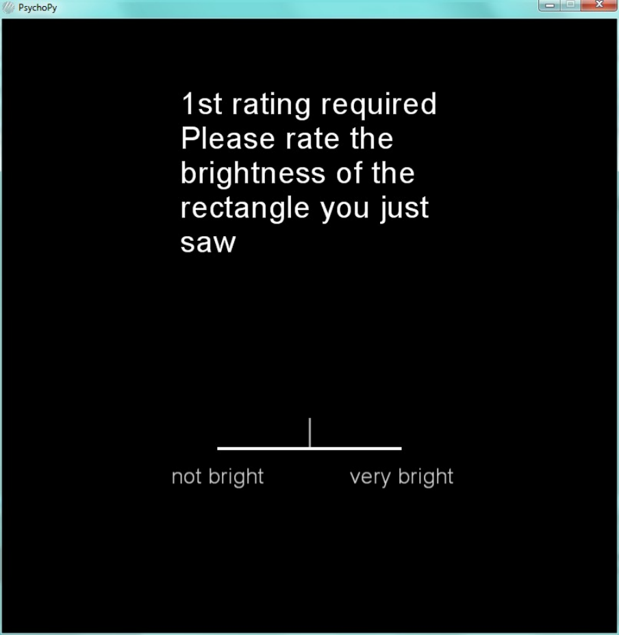
611

612

613
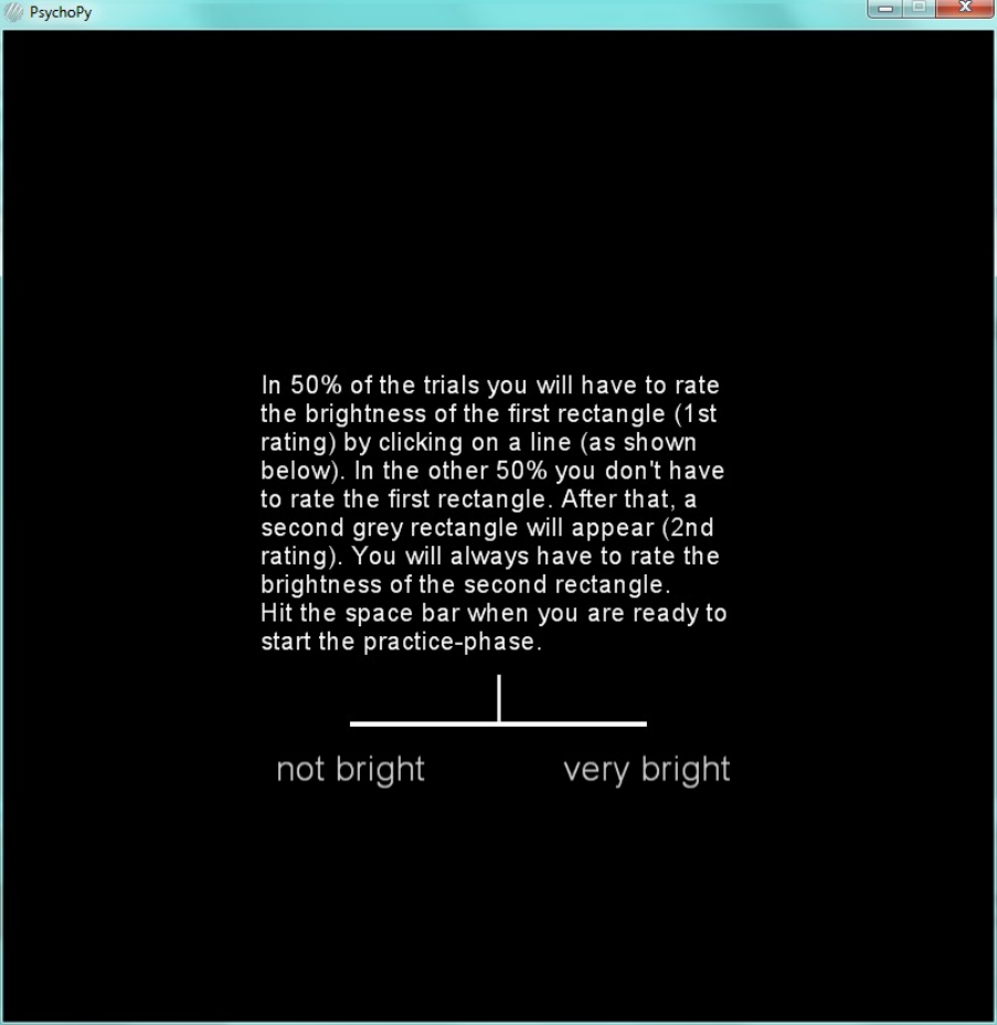
614

615

616

617

618

619

620

621

622
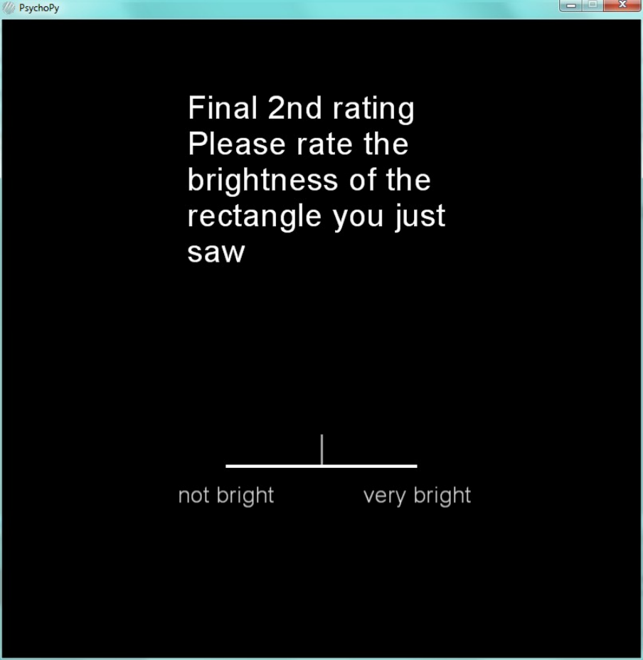
623

624

625
Debriefing
Debrief
Anonymous participant ID: _________________________
Thank you for participating in this study!
Your participation will help us to investigate order-effects in visual-decision making from a
quantum probability perspective.
What is quantum cognition?
Quantum cognition is a newly emerging paradigm within psychology and neuroscience
(Pothos & Busemeyer, 2013). It is based on the mathematical framework of quantum theory
which provides a general axiomatic theory of probability. This novel approach has the
potential to become a viable alternative to classical statistical models.
For general information visit:
http://en.wikipedia.org/wiki/Quantum_cognition
For in depth information we recommend the following paper which is freely available online
(see reference below):
http://openaccess.city.ac.uk/2428/
If you have any further questions, or if you want to withdraw you data, please feel free to
contact the researcher.
Researcher: Christopher Germann: christopher.germann@plymouth.ac.uk
Supervisor: Prof. Chris Harris: chris.harris@plymouth.ac.uk
References
Pothos, E. M., & Busemeyer, J. R. (2013). Can quantum probability provide a new
direction for cognitive modeling. Behavioral and Brain Sciences, 36, 255-274.
Q-Q plots
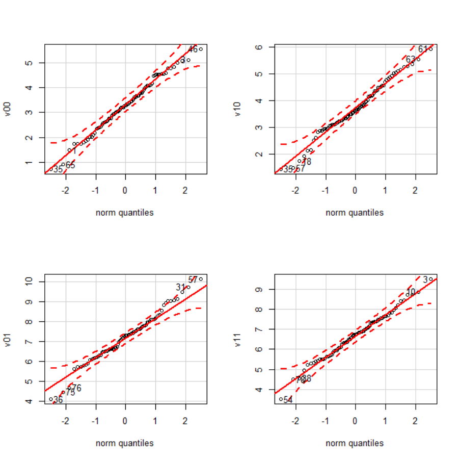
626
Figure 93. Q-Q plots identifying the 5 most extreme observation per experimental
condition (linearity indicates Gaussianity).

627
The Cramér-von Mises criterion
Equation 14. The Cramér-von Mises criterion (Cramér, 1936)
=
[
()
()]
d
()
The criterion can be used to as a goodness-of-index and it’s a viable alternative to the
more widely used Kolmogorov–Smirnov test. It is eponymously named after Harald
Cramér and Richard Edler von Mises who proposed it in 1928–1930.
Shapiro-Francia test
The Shapiro-Francia test is an analysis of variance test for normality and has good
statistical properties (see also the comments by Royston, 1993)
Equation 15. The Shapiro-Francia test (S. S. Shapiro & Francia, 1972)
=
cov (, )
=
(
)(
)
(
(
)
)(
(
)
)

628
Fisher’s multivariate skewness and kurtosis
Equation 16. Fisher’s multivariate skewness and kurtosis
Skewness = G1
Kurtosis = G2
=
(1)
2
/
,
=
1
(2)(3)
[(+ 1)(
3) + 6],
where
=
(
)
/
denotes the r
th
central moment, the sample mean, and n the sample size (Cain et al.,
2016).
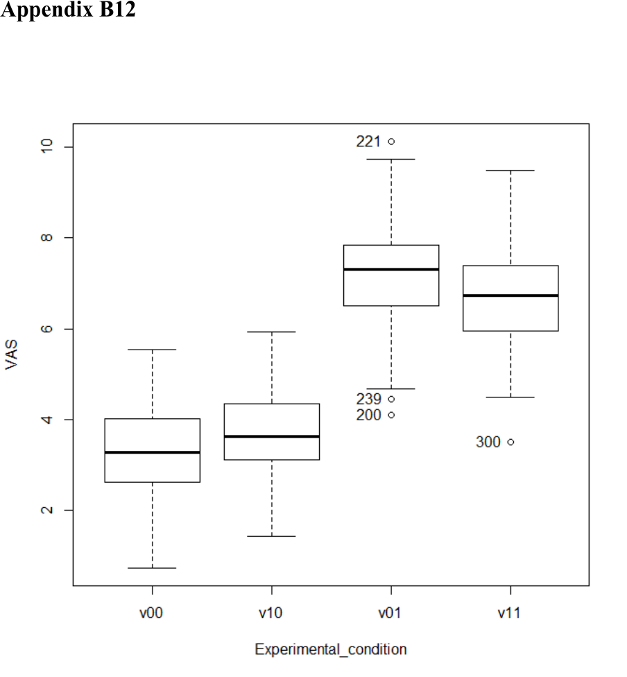
629
Median-based boxplots
Figure 94. Boxplots visualising differences between experimental conditions (i.e.,
median, upper and lower quartile).
Note that several potential outliers are identified (i.e., observation “200" "239" "221"
"300").

630
#https://cran.r-project.org/web/packages/beanplot/beanplot.pdf
par( mfrow = c( 1, 4 ) )
with(dataexp2, beanplot(v00, ylim = c(0,10), col="lightgray", main =
"v00", kernel = "gaussian", cut = 3, cutmin = -Inf, cutmax = Inf,
overallline = "mean", horizontal = FALSE, side = "no", jitter = NULL,
beanlinewd = 2))
with(dataexp2, beanplot(v01, ylim = c(0,10), col="lightgray", main =
"v01", kernel = "gaussian", cut = 3, cutmin = -Inf, cutmax = Inf,
overallline = "mean", horizontal = FALSE, side = "no", jitter = NULL,
beanlinewd = 2))
with(dataexp2, beanplot(v10, ylim = c(0,10), col="darkgray", main = "v10"
,
kernel = "gaussian", cut = 3, cutmin = -Inf, cutmax = Inf, overallline =
"mean", horizontal = FALSE, side = "no", jitter = NULL, beanlinewd = 2))
with(dataexp2, beanplot(v11, ylim = c(0,10), col="darkgray", main = "v11"
,
kernel = "gaussian", cut = 3, cutmin = -Inf, cutmax = Inf, overallline =
"mean", horizontal = FALSE, side = "no", jitter = NULL, beanlinewd = 2))
par( mfrow = c( 1, 2 ) ) ###############################################
with(dataexp2, beanplot(v00, col="darkgray", main = "v00", kernel =
"gaussian", cut = 3, cutmin = -Inf, cutmax = Inf , overallline = "mean",
horizontal = FALSE, side = "no", jitter = NULL, beanlinewd = 2))
with(dataexp2, beanplot(v01, col="darkgray", main = "v01", kernel =
"gaussian", cut = 3, cutmin = -Inf, cutmax = Inf , overallline = "mean",
horizontal = FALSE, side = "no", jitter = NULL, beanlinewd = 2))
par( mfrow = c( 1, 2 ) )
with(dataexp2, beanplot(v10, col="darkgray", main = "v10", kernel =
"gaussian", cut = 3, cutmin = -Inf, cutmax = Inf , overallline = "mean",
horizontal = FALSE, side = "no", jitter = NULL, beanlinewd = 2))

631
with(dataexp2, beanplot(v11, col="darkgray", main = "v11", kernel =
"gaussian", cut = 3, cutmin = -Inf, cutmax = Inf, overallline = "mean",
horizontal = FALSE, side = "no", jitter = NULL, beanlinewd = 2))
Code 5. R code for symmetric and asymmetric “beanplots”.

632
Tolerance intervals based on the Howe
method
The subsequent tolerance intervals (Krishnamoorthy & Mathew, 2008) are based on the
Howe method (Howe, 1969) and were computed using the “tolerance” R package
(Young, 2010). The tolerance interval defines and upper and lower bound between
which a given proportion β of the population lies with a prespecified confidence level
(1-α). Tolerance intervals circumvent the “robust misinterpretation of confidence
intervals”, that is, it has been empirically demonstrated that the majority of academics
misinterpret conventional confidence intervals (Hoekstra et al., 2014) which can lead to
wrong conclusions which can cause serious detrimental real-world consequences.
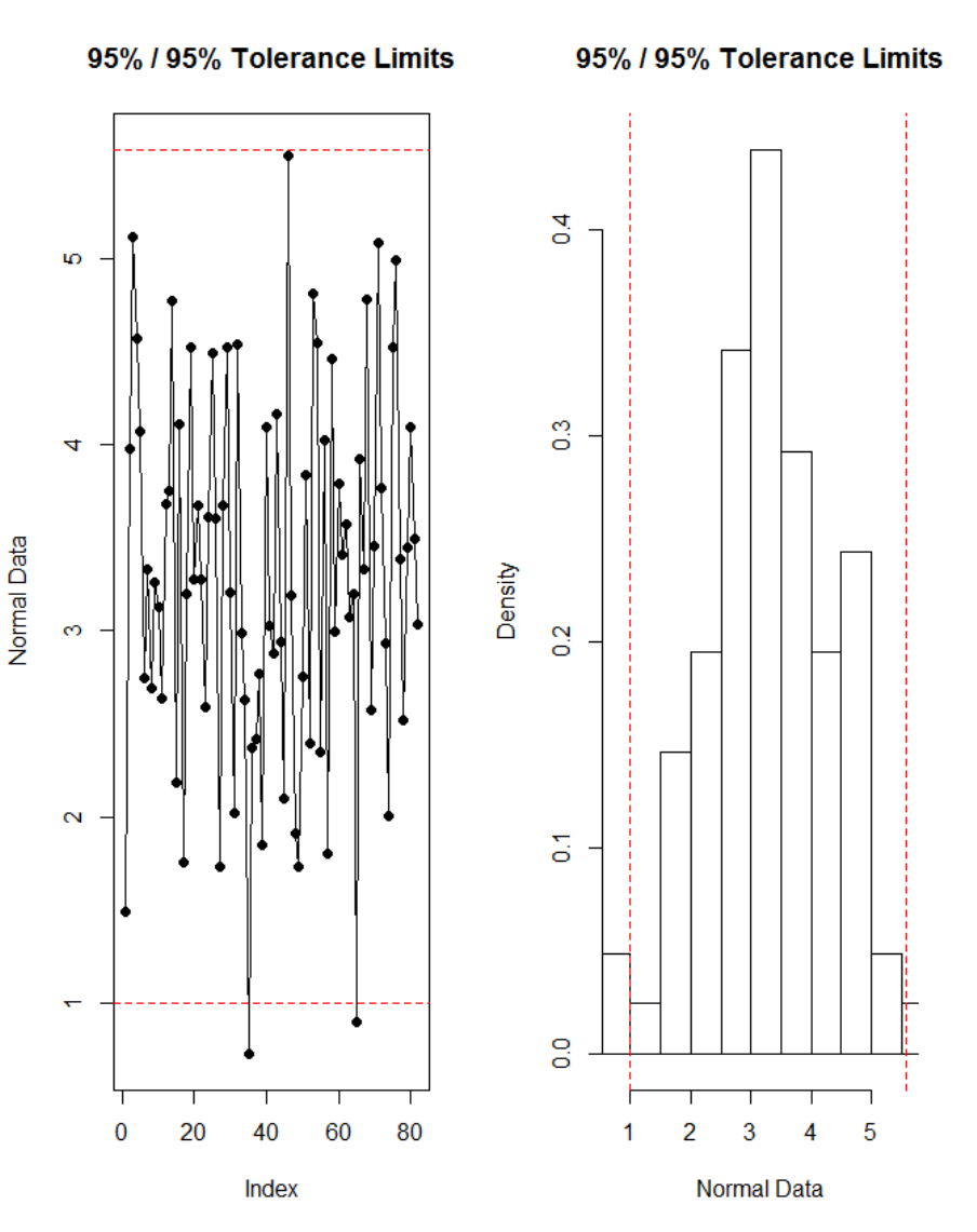
633
Figure 95. Tolerance interval based on Howe method for experimental condition V
00
.
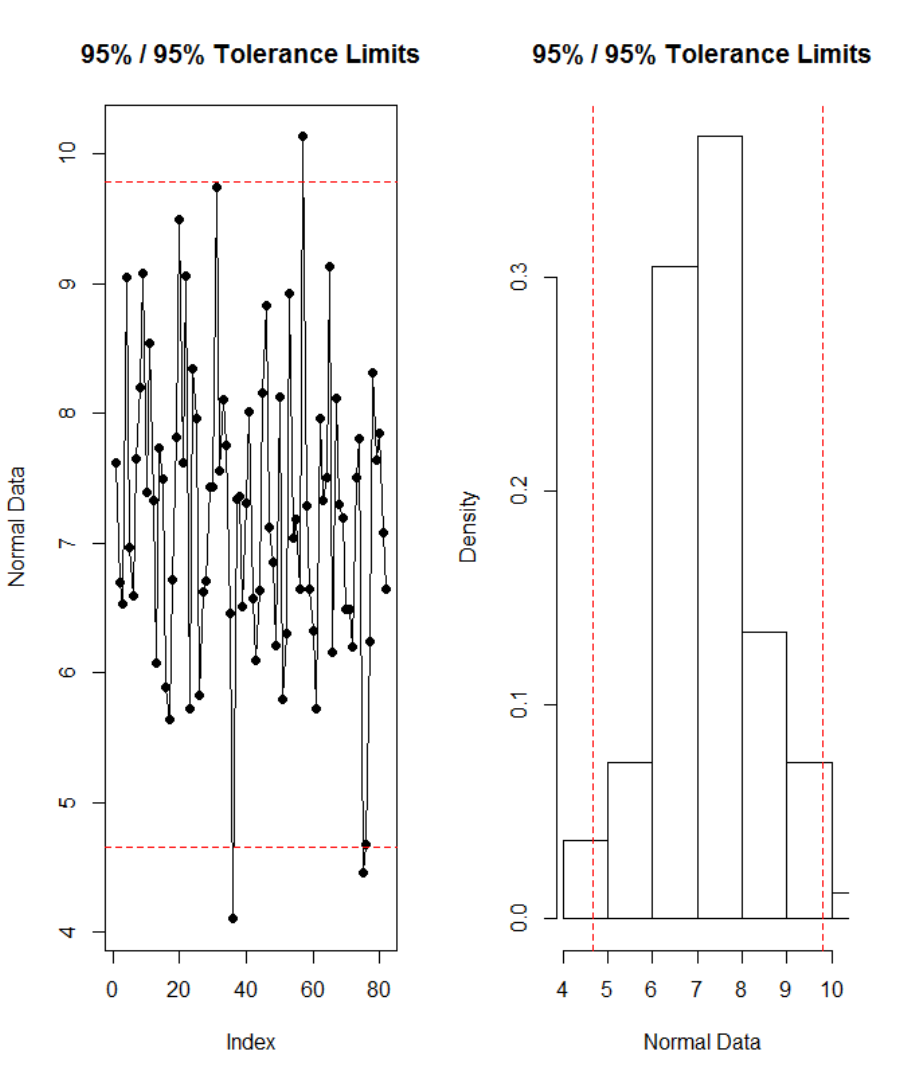
634
Figure 96. Tolerance interval based on Howe method for experimental condition V
01
.
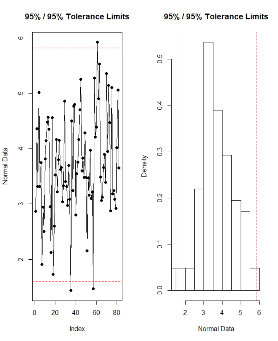
635
Figure 97. Tolerance interval based on Howe method for experimental condition V
10
.
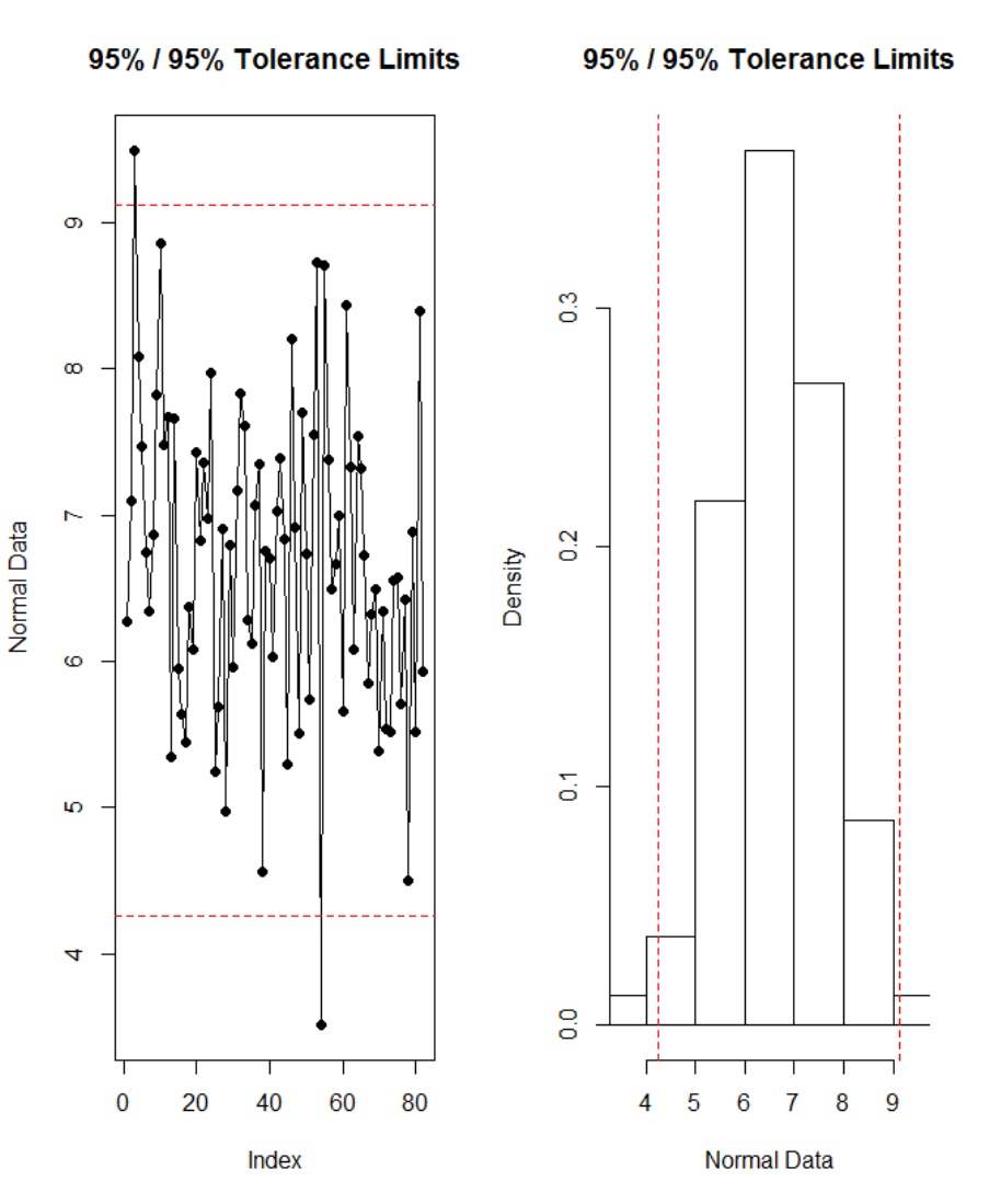
636
Figure 98. Tolerance interval based on Howe method for experimental condition V
11
.

637
Alternative effect-size indices
It has been noted that “reporting of effect size in the psychological literature is patchy”
(Baguley, 2009a, p. 603) even though it is regarded as “best practice” in quantitative
research. The decision which effect size metric to report require careful consideration.
This can be an issue, given that effortful decision deplete cognitive resources
(Baumeister, Vohs, & Tice, 2007).
Even though heuristic “rules of thumb” have been suggested some statistically well
versed researchers argue that "canned effect sizes” (Baguley, 2009a, p. 613). This
especially true for psychophysical research where differences are often minute but still
meaningful. We argue, that effect sizes should be evaluated in context. There are no
mechanistic decision-procedures for the classification of effect sizes. These values are
always situated and statistical reflection (i.e., cognitive effort) is indispensable.
Heuristics vs. analytics: dual system approach (Kahneman, 2003).
Based on Monte Carlo simulations, it has been argued that in order to estimate δ from
empirical data, Hedges’s g is regarded as superior to the more widely reported Cohen’s
d (Kelley, 2005). The formulaic descriptions of several effect-size metrics are given
below.
Equation 17: Cohen's d (Cohen, 1988)
=
=
.
=
(
1)
+ (
1)
+
2

638
=
1
1
(
,
)
,
Equation 18: Glass' Δ (Glass, 1976)
=
Equation 19: Hedges' g (Hedges, 1981)
=
=
(
)
(
)
.
signifies the pooled and weighted standard deviation. Hence, the defining difference
between Hedge’s g and Cohen’s d is that the former integrates pooled weighted
standard deviations, whereas the later uses the pooled standard deviations). Whenever
standard deviations differ “substantially” between conditions, Glass's Δ should be
reported

639
Nonparametric bootstrapping
We used nonparametric bootstrapping techniques in order to check the robustness and
stability of our results and to maximise statistical inferential power. We performed a
bootstrap using the “boot” package (Canty & Ripley, 2012) in R for the t-tests and the
“BootES” package (Kirby & Gerlanc, 2013) for the effect sizes and their associated
confidence intervals. We obtained bootstrapped confidence intervals for all parameters
of interest. Bootstrapping simulations (i.e. resampling with replacement) is a powerful
method which facilitates more accurate statistical inferences compared to conventional
NHST methods (e.g., bootstrapping is asymptotically more accurate relative to standard
CIs based on the Gaussianity assumption and using sample variance). Bootstrap
methods do not rely on any assumption regarding the parent distribution from which the
bootstrap samples are drawn. As such, bootstrapping “can be remarkably more accurate
than classical inferences based on Normal or t distributions” (Hesterberg, 2011, p. 497).
The growing popularity of this powerful statistical methodology is linked to recent
advances in computational capacities because bootstrapping can be computationally
demanding.
237
We choose rather large numbers of bootstrap samples for our analysis
(i.e., 100000 replicates per simulation) in order to achieve a high degree of precision.
237
We utilised an Intel® Core™ i7-2600 processor @ 3.40GHz with 16GB RAM for the reported
bootstrap simulations.
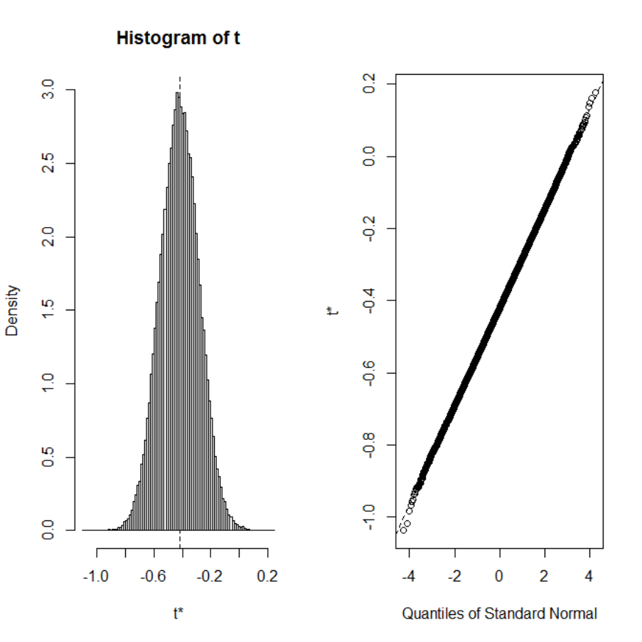
640
Figure 99. Bootstrapped mean difference for experimental conditions V
00
vs. V
10
based
on 100000 replicas.
The QQ-plot indicates that the Gaussian distribution has been achieved (due to the
central limit theorem), i.e., the number of bootstrap resamples R is large enough to
obtain parameter estimates with high accuracy.
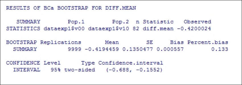
641
Table 42
Results of Bca bootstrap analysis (experimental condition V
00
vs. V
10
).

642
Figure 100. Bootstrapped mean difference for experimental conditions V
10
vs. V
11
based
on 100000 replicas.
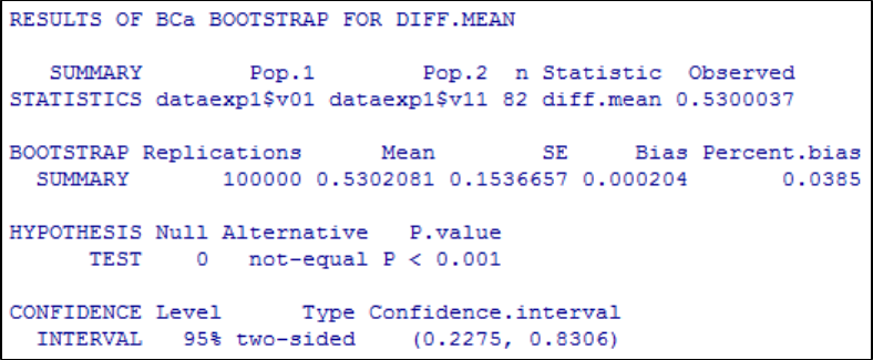
643
Table 43
Results of Bca bootstrap analysis (experimental condition V
10
vs. V
11
).
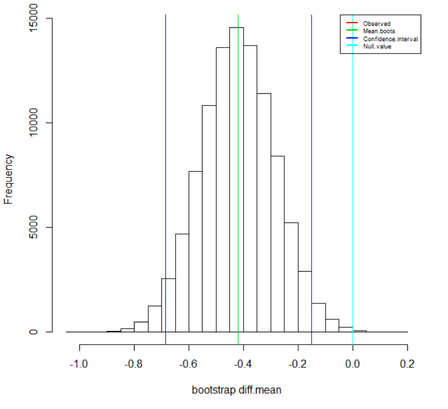
644
Figure 101. Histogram of the bootstrapped mean difference between experimental
condition V
00
and V
10
based on 100000 replicates (bias-corrected & accelerated) with
associated 95% confidence intervals.
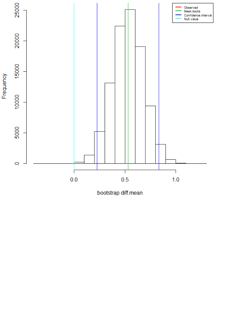
645
Figure 102. Histogram of the bootstrapped mean difference between experimental
condition V
01
and V
11
based on 100000 replicates (bias-corrected & accelerated) with
associated 95% confidence intervals.
We applied the BCa (bias-corrected & accelerated) bootstrap to the data (Harald Steck
& Jaakkola, 2003). Computations are based on R=100000 bootstrap replicates. BCa
method for computing bootstrap CIs, which has been shown to have excellent coverage
in a wide. For both normal and nonnormal population distributions with sample sizes of
roughly 20 or more, Monte Carlo research has shown that BCa intervals yield small

646
coverage errors for means, medians, and variances (Lei & Smith, 2003), correlations
(Padilla & Veprinsky, 2012), and Cohen’s d (Algina, Keselman, & Penfield, 2006). The
magnitude of the coverage errors, and whether they are liberal or conservative, depends
on the particular statistic and the population distribution, and BCa intervals can be
outperformed by other methods in particular circumstances (Hess, Hogarty, Ferron, &
Kromrey, 2007). In sum, the results confirm corroborate the robustness of our previous
analyses.
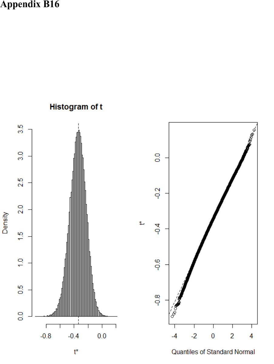
647
Bootstrapped effect sizes and 95% confidence
intervals
In addition we employed the “BootES” package (Kirby & Gerlanc, 2013) in R to
bootstrap the confidence intervals of the effect size (i.e, Cohens d).
Figure 103. Bootstrapped effect size (Cohen’s d) for condition V
00
vs V
01
based on
R=100000.
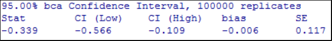
648
Numerical results:

649
Figure 104. Bootstrapped effect size (Cohen’s d) for condition V
10
vs V
11
based on
R=100000.
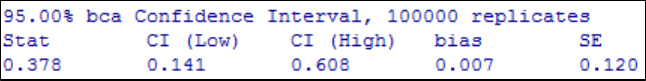
650
Numerical results:
The bootstraps corroborate the previously reported effect sizes, thereby providing
additional evidence for the robustness and stability of the results. The bootstrapped bias
corrcted & accelerated 95% confidence intervals provide a higher degree of statistical
precision than the previous NHST analysis did (cf. Table 3).

651
Bayesian bootstrap
Given the logical shortcomings and ubiquitous misinterpretations associated with NHST
confidence intervals (Hoekstra et al., 2014), we performed a Bayesian bootstrap with
associated high density intervals (Silverman, 1986). Bayesian high density intervals
provides much more detailed information than conventional frequentist confidence
intervals do (Kruschke, 2015; Kruschke & Liddell, 2017c) and they are not inherently
prone to logical misapprehension. For this analytic purpose, we utilised the
“bayesboot” package
238
in R which provides an implementation of the Bayesian
bootstrap
239
formalised by Rubin (1981). We fixed the size of the posterior sample from
the Bayesian bootstrap to 100000 in order to achieve a high degree of statistical
accuracy. Moreover, we utilised the implemented “parallel processing” functionality of
the “plyr” package (Wickham, 2014) in order to boost the speed of the simulations.
First, we computed Bayesian bootstraps for means per experimental condition. The
density estimates for experimental condition V
00
and V
10
are combined in Figure 105
and numerical summery is given in
238
The “bayesboot” package for R can be downloaded from the collaborative GitHub open-source
(crowdsourced) software repository (Bååth, 2012) under the following URL:
https://github.com/rasmusab/bayesboot
Unfortunately, there are currently no naming conventions in R
which renders the declaration of variables and functions somewhat arbitrary (cf. Kahneman & Tversky,
1974).
239
The underlying model can be formalised as follows:
} for in 1..N 1
Categorical
(
)
} for in 1..N 1
Dirichlet(0
, … , 0
)
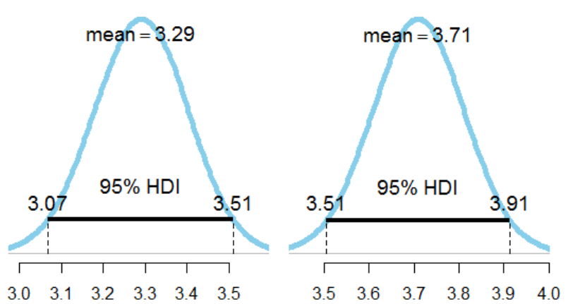
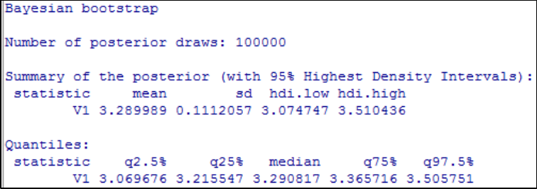
653
Table 44
Numerical summary of Bayesian bootstrap for condition V
00
.
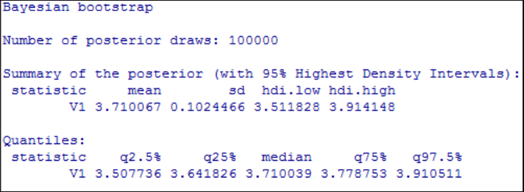
654
Table 45
Numerical summary of Bayesian bootstrap for condition V
10
.

655
In sum, the results indicate that the Bayesian bootstrapped posterior mean estimate for
condition V
00
is 3.29 with a 95% HDI
240
ranging from [3.07, 3.51]. The bootstrapped
posterior mean of condition V
10
was estimated to be 3.7 with a 95% HDI spanning from
[3.51, 3.91]. In contrast to NHST confidence intervals, the HDI indicates that there is a
95% probability that the “true” value of the mean lies within the boundaries of the
respective interval (Kruschke & Liddell, 2017b). That is, it can be concluded that there
is a 95% probability that the credible mean for condition V
00
lies between the infimum
of 3.07 and the supremum of 3.51. This kind of probabilistic conclusion cannot be
derived from classical frequentist confidence intervals — even though they are
evidently ubiquitously fallaciously misinterpreted in this way by the majority of
academic researchers
241
(Hoekstra et al., 2014).
240
The HDI summarizes the distribution by specifying an interval that spans most of the distribution, say
95% of it, such that every point inside the interval has higher believability than any point outside the
interval. Its high dimension counterpart is HDR (high density region; a region can be n-dimensional
whereas an interval is by definition unidimensional). However, in the context at hand, we are primarily
concerned with single (one-dimensional) parameters.
241
Invalid logical conclusions can have large ramification because they necessarily lead to irrational
decisions. Ergo, it is pivotal that researchers utilise analytic methods that are not prone to international
biases (cf. Ioannidis, 2005). The decisions researchers base on their (il)logical analytical conclusions
oftentimes have far reaching real-world consequences and the implications of such cognitive biases
should not be taken lightly (Goldstein, 2006).
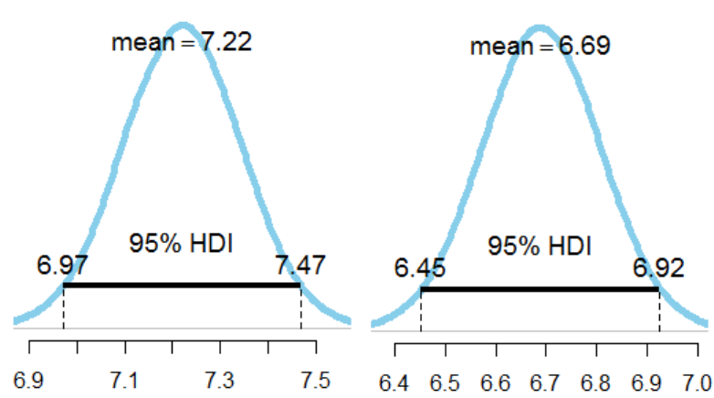
656
Next, we conducted Bayesian bootstraps for experimental conditions V
01
and V
11
. The
results indicate that the bootstrapped posterior mean for condition V
01
is 7.22 with a
95% HDI ranging from [6.97, 7.47], whereas the mean of condition V
11
was 6.69 with a
95% HDI spanning from [6.45, 3.92].
Figure 106. Posterior distributions (based on 100000 posterior draws) for experimental
conditions V
01
and V
11
with associated 95% high density intervals.
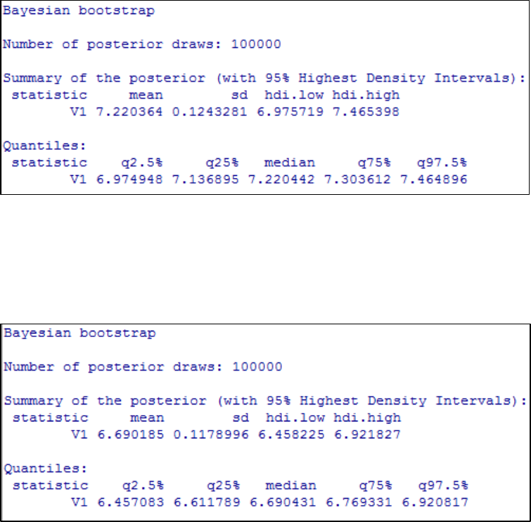
657
Table 46
Numerical summary of Bayesian bootstrap for condition V
01
.
Table 47
Numerical summary of Bayesian bootstrap for condition V
11
.
Finally, we computed Bayesian bootstraps for the mean difference between condition in
order to explicitly evaluate our a priori hypotheses. The density estimates of the first
analysis, comparing conditions V
00
vs. V
10
, are visualised in
Figure 107 and a histogram of the posterior distribution is provided in
Figure 108. Posterior distribution (n=100000) of the mean difference between V00 vs.
V10.
In addition, a numerical summary is given in
658
Table 48. From this analysis it can be concluded that the mean difference between
experimental condition V
00
vs. V
10
is ≈-0.42with a 95% HDI spanning from [-0.72, -
0.12]. In other terms, there is a 95% probability that the credible value of the mean lies
between -0.72 and -0.12. Furthermore, it can be concluded that the estimated probability
that the mean difference between experimental condition V
01
vs. V
11
is < 0 is exactly
0.9975012. In addition, we construted a region of practical equivalence (ROPE) around
the comparison value of zero (referring to H
0
). In
Figure 107, the comparison value is shown as a vertical green dashed line and the
ROPE is demarcated by red vertical dashed lines. Prima vista, it can be seen that the
probability mass within the ROPE is 2% and that the probability mass above and below
the comparison value is 99.7% < 0 < 0.3. Given that the ROPE lies entirely outside the
HDI, H
0
can be rejected (Kruschke, 2014).
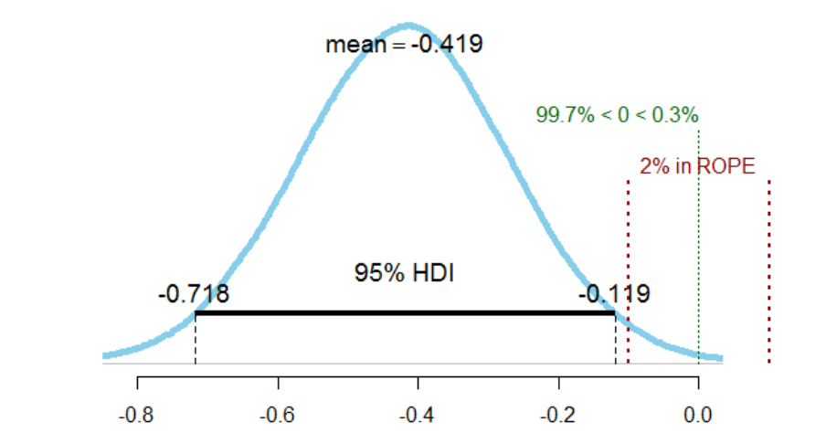
659
Figure 107. Histogram of the Bayesian bootstrap (R=100000) for condition V
00
vs. V
10
with 95% HDI and prespecified ROPE ranging from [-0.1, 0.1].
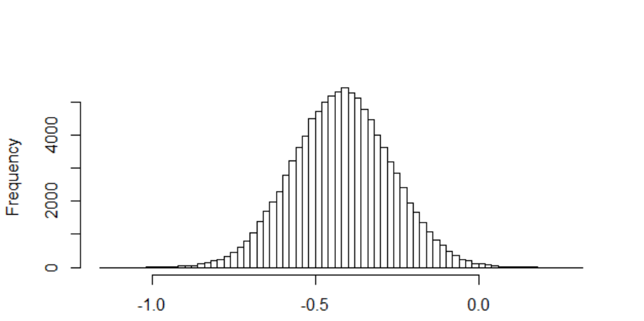
660
Figure 108. Posterior distribution (n=100000) of the mean difference between V
00
vs.
V
10.
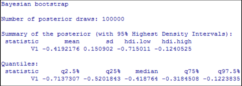
661
Table 48
Numerical summary of Bayesian bootstrap for the mean difference between V
00
vs. V
10
.
We repeated the same analysis for the mean difference between experimental condition
V
01
vs. V
11
. A visual synopsis is given in Figure 109. The associated posterior
distribution is plotted in Figure 109.
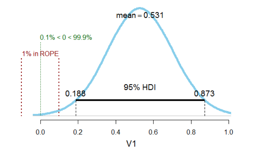
662
Figure 109. Histogram of the Bayesian bootstrap (R=100000) for condition V
01
vs. V
11
with 95% HDI and prespecified ROPE ranging from [-0.1, 0.1].
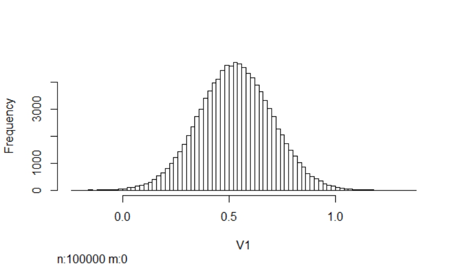
663
Figure 110. Posterior distribution (n=100000) of the mean difference between V
01
vs.
V
11.
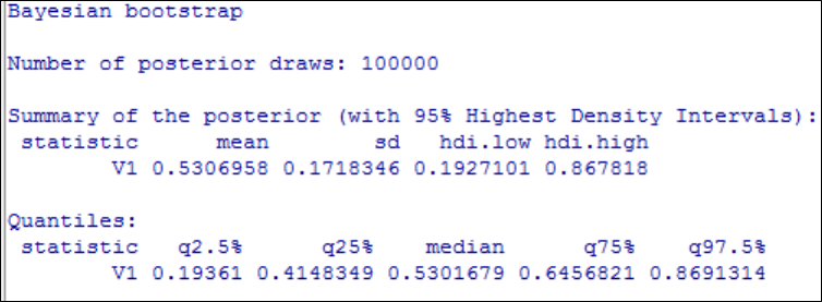
664
Table 49
Numerical summary of Bayesian bootstrap for the mean difference between V
00
vs. V
10
.
The probability that the mean difference between experimental condition V
01
vs. V
11
is
> 0 is exactly 0.99907.
665
In sum, the Bayesian bootstrap corroborated the conclusions derived from the results of
our initial frequentist analysis and provided additional new information which was
unavailable in the NHST framework. The analysis provided a methodological cross-
validation and confirmed the robustness of our results. Moreover, the Bayesian
bootstrap approach allowed us to compute 95% high density intervals which were
utilised in combination with ROPEs to test our hypotheses. The results of the Bayesian
bootstrap converged with those of the classical parametric bootstrap. This is generally
the case with large samples and the results of the parametric bootstrap can thus be
interpreted in a Bayesian framework if n is sufficiently large (with smaller samples the
results generally diverge). However, it should be noted that the Bayesian bootstrap (and
the classical non-parametric bootstrap) make some assumptions which are questionable
and not necessarily appropriate. For instance, it is assumed:
• That values not observed before are impossible
• That values outside the range of the empirical data are impossible
It has been asked before: “…is it reasonable to use a model specification that effectively
assumes all possible distinct values of X have been observed?” (D. B. Rubin, 1981).

666
Probability Plot Correlation Coefficient
(PPCC)
Summary of the results of the “Probability Plot Correlation Coefficient” test (Looney &
Gulledge, 1985) using the “PPCC”
242
R package. The PPCC computes a goodness-of-fit
index
^
for various distributions (Hanson & Wolf, 1996). Hence, it can be utilised to
evaluate normal and non-normal distributional hypotheses. Each PPCC test was
performed with 10000 Monte-Carlo simulations. The results indicated Gaussianity for
all conditions. The PPCC is mathematically defined as the product moment correlation
coefficient between the ordered data x
(i)
and the order statistics medians M
i
, whereas the
ordered statistic medians are related to the quantile function of the standard normal
distribution,
=
(
).
Equation 20. Probability Plot Correlation Coefficient (PPCC)
=
(
)
~
(
)
(
)
~
,
242
Available on CRAN: https://cran.r-project.org/web/packages/ppcc/ppcc.pdf

667
Table 50
Results of PPCC analysis (based on 10000 Monte-Carlo simulations).
data: dataexp1$v00
ppcc = 0.9966, n = 82, p-value = 0.9091
alternative hypothesis: dataexp1$v00 differs from a Normal distribution
data: dataexp1$v01
ppcc = 0.99195, n = 82, p-value = 0.3399
alternative hypothesis: dataexp1$v01 differs from a Normal distribution
data: dataexp1$v10
ppcc = 0.99319, n = 82, p-value = 0.4643
alternative hypothesis: dataexp1$v10 differs from a Normal distribution
data: dataexp1$v11
ppcc = 0.99557, n = 82, p-value = 0.7864
alternative hypothesis: dataexp1$v11 differs from a Normal distribution
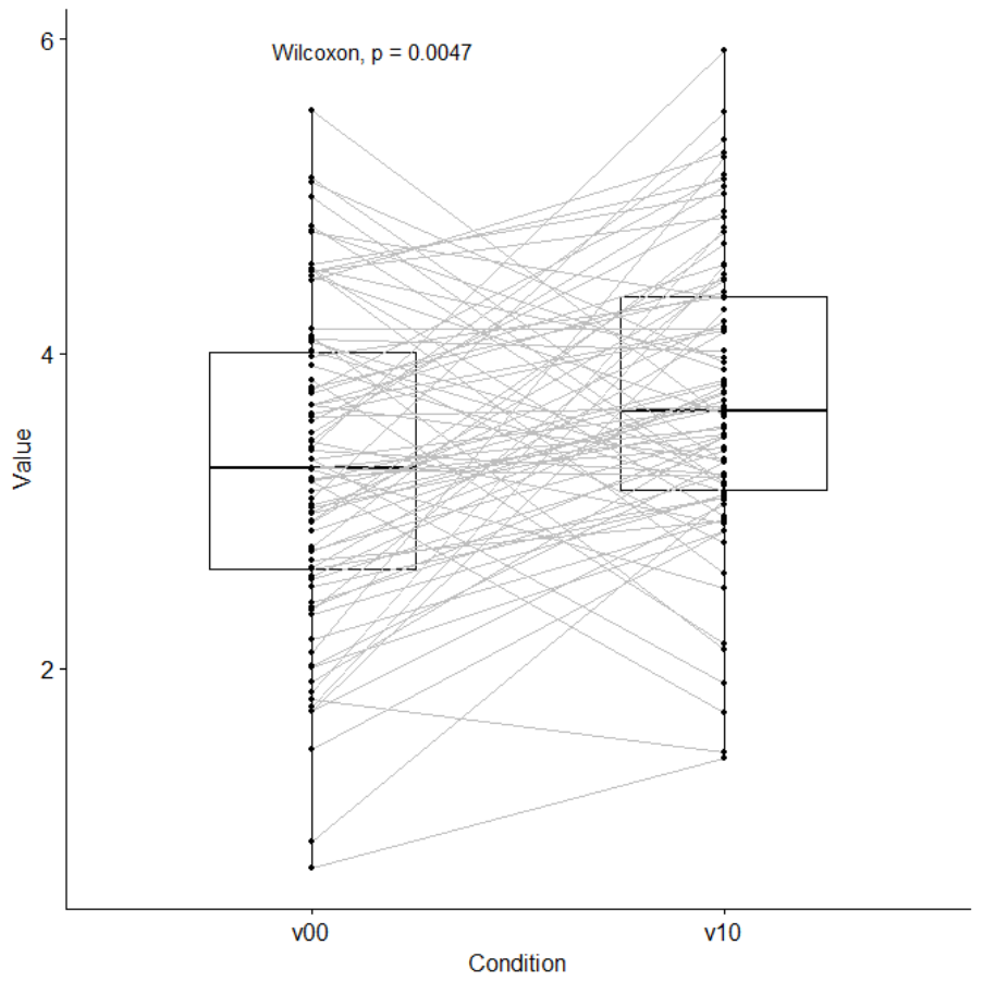
668
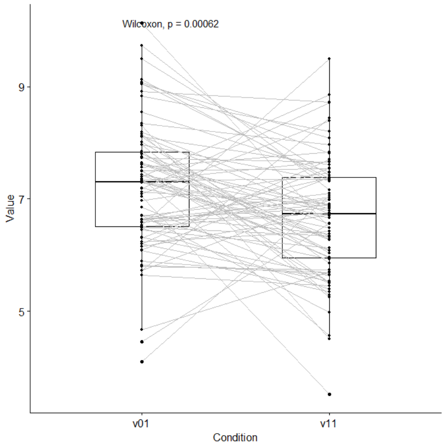
669
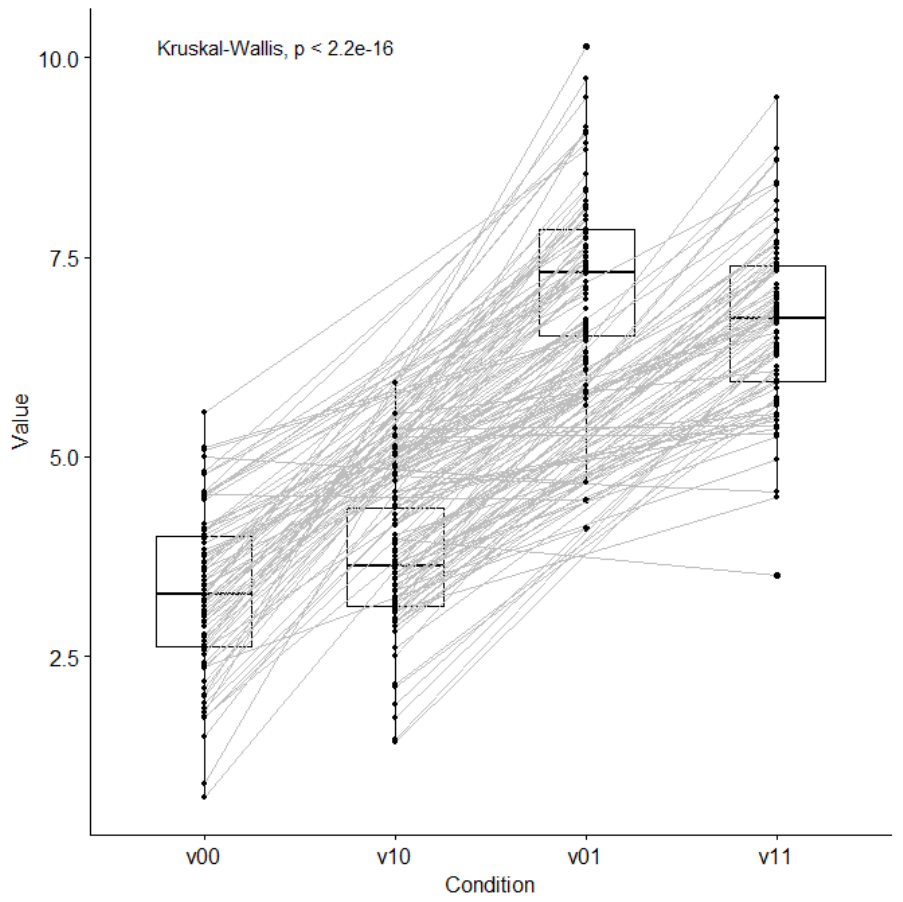
670

671
Ngrams for various statistical methodologies

672
Bayes Factor analysis (supplementary
materials)
In physics the Cauchy distribution (CD) is also termed Lorentz or Breit-Wigner
distribution, and it has many applications in particle physics. Cauchy distribution is a t
distribution with 1 degree of freedom and due to its shape (it belongs to the class of
heavy-tailed distribution, see Figure 111 below) it has no determinable mean and an
infinite variance (Rouder et al., 2009). Hence it is also called a “pathological"
distribution. It has been pointed out that Bayes factors with the Cauchy prior are slightly
biased towards H
0
(Rouder et al., 2009), i.e., the Cauchy prior is slightly conservative
towards H
1
.
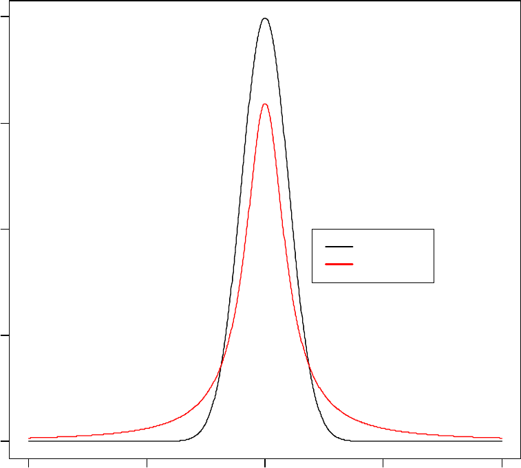
673
Figure 111. Visual comparison of Cauchy versus Gaussian prior distributions
symmetrically centred around δ. The abscissa is standard deviation and ordinate is the
density.
-10
-5
0 5 10
0.0 0.1 0.2 0.3 0.4
x
dnorm
Gaussian
Cauchy

674
plot(dnorm, -10, 10, n=1000)
plot(dcauchy, -10, 10, n=1000, col='red', add=TRUE)
legend(0.01,0.01, c("Gaussian","Cauchy"),
lty=c(1,1,1),
lwd=c(2,2,2), col=c("black", "red"))
Code 6. R code for plotting Cauchy versus Gaussian distribution (n=1000)
symmetrically centred around δ [-10,10].
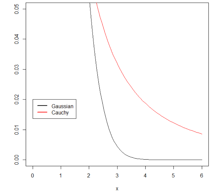
675
Figure 112. Graphic of Gaussian versus (heavy tailed) Cauchy distribution. X axis is
standard deviation and y axis is the density

676
low <- 0; high <- 6
curve(dnorm,from = low, to = high, ylim = c(0, .05), col = "blue", ylab = "
", add = FALSE)
curve(dcauchy,from = low, to = high, col = "red", add = TRUE)
plot(dnorm, -10, 10, n=1000)
plot(dcauchy, -10, 10, n=1000, col='red', add=TRUE)
legend(0,0.02, c("Gaussian","Cauchy"),
lty=c(1,1,1), # symbols (lines)
lwd=c(2,2,2), col=c("black", "red"))
legend(0,0.03, c("Gaussian","Cauchy"),
lty=c(1,1,1), # symbols (lines)
lwd=c(2,2,2), col=c("blue", "red"))
Code 7. R code for plotting tails of Cauchy versus Gaussian distributions.
677
The Cauchy distribution is a t distribution with a single degree of freedom. It has tails so
heavy that neither its mean nor its variance exist. A comparison of the Cauchy prior to
the unit-information prior is shown in Figure 3B. As can be seen, the Cauchy allows for
more mass on large effects than the standard normal. Consequently, Bayes factors with
the Cauchy prior favour the null a bit more than those with the unit-information prior.
The JZS prior is designed to minimize assumptions about the range of effect size, and in
this sense it is an objective prior. Smaller values of r, say 0.5, may be appropriate when
small effect sizes are expected a priori; larger values of r are appropriate when large
effect sizes are expected. The choice of r may be affected by theoretical considerations,
as well: Smaller values are appropriate when small differences are of theoretical
importance, whereas larger values are appropriate when small differences most likely
reflect nuisances and are of little theoretical importance. In all cases, the value of r
should be chosen prior to analysis and without influence from the data. In summary, r 5
1.0 is recommended (serves as a benchmark) - surreptitiously choosing a self-serving
prior - This appearance is deceiving. Bayes factors are not particularly sensitive to
reasonable variation in priors, at least not with moderate sample sizes. (Berger & Berry,
1988)
It is reasonable to ask whether hypothesis testing is always necessary. In many ways,
hypothesis testing has been employed in experimental psychology too often and too
hastily, without sufficient attention to what may be learned by exploratory examination
for structure in data (Tukey, 1977). To observe structure, it is often sufficient to plot
estimates of appropriate quantities along with measures of estimation error (Rouder &
Morey, 2005). As a rule of thumb, hypothesis testing should be reserved for those cases
in which the researcher will entertain the null as theoretically interesting and plausible,
at least approximately. Researchers willing to perform hypothesis testing must realize
678
that the endeavor is inherently subjective and objectivity is illusionary, (as might be the
objectivity of science in general as argued by ) (Irwin & Real, 2010). Moreover; similar
unconscious biases as those observed in legal decision making might apply (but see
Molloy, 2011)
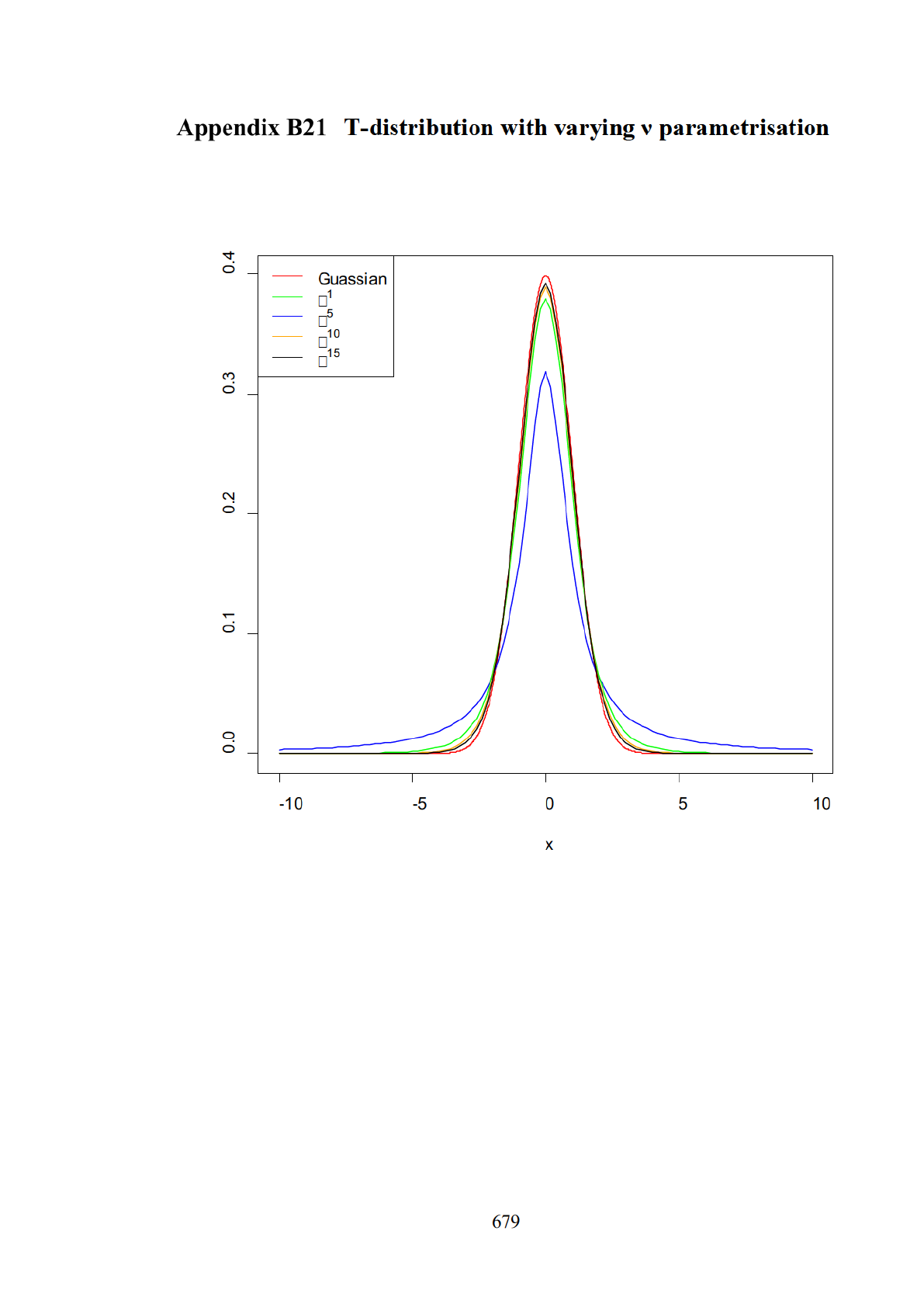
6 7 9
T- dist ri b uti o n wit h v a r yi n g ν p a r a m et ris ati o n
- 1 0 - 5 0 5 1 0
0. 0 0. 1 0. 2 0. 3 0. 4
x
G u a s s ia n
1
5
1 0
1 5

680
#t distribution with varying nu parametrisation
curve(dnorm(x), -10, 10, n=1000, col = "red", ylab="")
curve(dt(x, df = 1), col = "blue", add = TRUE)
curve(dt(x, df = 5), col = "green", add = TRUE)
curve(dt(x, df = 10), col = "orange", add = TRUE)
curve(dt(x, df = 15), col = "black", add = TRUE)
legend_texts = expression(
Guassian, nu^1, nu^5, nu^10, nu^15)
legend("topleft",legend = legend_texts, col = c("red", "green", "blue",
"orange", "black"), lty = c(1))
Code 8. R code for plotting t-distributions with varying ν parametrisation.
In R, the density of t at x is determined by dt(x,df), where df is the parameter for the
degrees of freedom. Note, that the degrees of freedom are not related to a sampling
distribution. Here df is not restricted to being an integer (Kruschke, 2010a).

681
Evaluation of null-hypotheses in a Bayesian
framework: A ROPE and HDI-based decision algorithm
In the majority of psychological research is it is conventional to try to reject H
0
.
Bayesian parameter estimation can likewise be utilised to assess the credibility of a
given null hypotheses (e.g., μ
1
– μ
2
= 0). This can be achieved by examining the
posterior distribution of the plausible parameter values (i.e., one simply checks if the
null value lies within the credible interval of θ). If the null value departs from the most
credible parameter value estimates it can be rejected in the classical Popperian sense
(Meehl, 1967; Rozeboom, 2005; Steiger, 2004). By contrast, if the credible values are
almost identical to the null value than H
0
can also be accepted, in contrast to the
asymmetry inherent to NHST. To be more explicit, Bayesian parameter estimation
methods allow the researcher to accept and reject a null value. Hence it can be regarded
as a symmetrical hypothesis testing procedure.
Another significant logical problem associated with NHST is that alternative theories
can be expressed very imprecisely (if at all) and still be “corroborated” by rejection of
H
0
. A problem known in philosophy of science as “Meehls’ paradox” (Carlin, Louis, &
Carlin, 2009), named after the ingenious psychologist and former APA president Paul
Meehl (see Rozeboom, 2005; Steiger, 2004). Differences of means that are
infinitesimally larger than zero can become statistically significant if n is large enough.
That is, given a large enough sample, any magnitude of difference can be considered
statistically significantly greater than zero. Bayesian parameter estimation provides
methods to circumvent this particular issue by constructing a region of practical
equivalence (ROPE) around the null value (or any other parameter of interest). The
ROPE is a bipolar interval that specifies a predefined range of parameter values that are
regarded as compatible with H
0
. In other words, the definition of the ROPE depends on
682
the experiment at hand and it involves a subjective judgment on the part of the
investigator. As n → ∞, the probability that the difference of means is exactly zero is
zero. Of theoretical interest is the probability that the difference may be too small to be
of any practical significance. In Bayesian estimation and decision theory, a region of
practical equivalence around zero is predefined. This allowed to compute the exact
probability that the true value of the difference lies inside this predefined interval
(Gelman et al., 2004). In the psychophysics experiment at hand, a difference of ± 0.01
in the visual analogue scale ratings was considered too trivial to be of any theoretical
importance (ergo, the a priori specified ROPE ranged from [-0.01;0,01]).
In addition to parameter estimation, the posterior distribution can be utilised to make
discrete decisions about specific hypotheses. High Density Intervals contain rich
distributional information about parameters of interest. Moreover, a HDI can be utilised
to facilitate reasonable decisions about null values (i.e., the null hypothesis that there is
no difference between condition V
00
and V
01
). HDIs indicate which values of θ are most
credible/believable. Furthermore, the HDI width conveys information regarding the
certainty of beliefs in the parameter estimate, i.e., it quantifies certainty vs. uncertainty.
A wide HDI is signifies a large degree of uncertainty pertaining to the possible range of
values of θ, whereas a narrow HDI indicates a high degree of certainty with regards to
the credibility of the parameters in the distribution. It follows, that the analyst can
define a specific degree of certainty by varying the width of the HDI. In other words,
the HDI entails the assembly of most likely values of the estimated parameters. For
instance, for a 95% HDI, all parameter values inside the interval (i.e., 95% of the total
probability mass) have a higher probability density (i.e., credibility/trustworthiness)
relative to those outside the interval (5% of the total mass). Moreover, the HDI contains
valuable distributional information, I n contrast to classic frequentists confidence

683
intervals (CI). For a classical 95% CI, all values within its range are equally likely, i.e.,
values in the centre of the confidence interval are equally like as those located at the
outer extremes. Furthermore, the range of 95% CI does not entail 95% of the most
credible parameter values. The choses terminology is in actuality very misleading as it
gives the impression that the 95% CI carries information about the confidentiality of the
values it entails (which it does not) The related widely shared logical fallacies are
discussed in chapter xxx. The Bayesian HDI does what the CI pretends to do. For
example, a 95% HDI is based on a density distribution, meaning that values in its centre
are more likely than those at the margin, viz., the total probability of parameter values
within the HDI is 95%. The HDI encompasses a large number of parameter values that
are jointly credible, given the empirical data. In other terms, the HDI provides
distributions of credible values of θ, not merely point estimates as is the case with CIs.
Thus, the HDI can be considered as a measure of precision of the Bayesian parameter
estimation it provides a summary of the distribution of the credible values of θ. Another
major advantage of HDIs over Cis is their insensitivity with regards to sampling
strategies and other data-collection idiosyncrasies that distort (and oftentimes logically
invalidate) the interpretation of p-values, and therefore Cis (which are based on p
values). The statistical inadequacies of CIs (which are nowadays advertised as an
integral part of “the new statistics”) are discussed in greater detail in chapter xxx.
The specified HDI can also be utilised in order to decide which values for θ are credible
(given the empirical data). For this purpose, a “Region of Practical Interest” (ROPE)
243
is constructed around the value of θ. Consider a ROPE for θ = 0 (i.e., μ
1
– μ
2
= 0) is
defined. The 95% ROPE defines a narrow interval which specifies values that are
243
The literature contains a multifarious nomenclature to refer to “regions of practical equivalence”.
Synonymous terms are, inter alia: “smallest effect size of interest”, “range of equivalence,” “interval of
clinical equivalence,” and “indifference zone,” etcetera (but see Kruschke & Liddell, 2017b).
684
deemed equivalent to θ = 0. That is, for all practical purpose, values that lie within the
Region of Practical Interest are regarded as equivalent to θ = 0. The ROPE procedure
allows flexibility in decision-making which is not available in other conventional
procedures (e.g., NHST). Another significant advantage is that no correction for
multiple comparisons are needed because no p values are involved. In other words, the
analysis does not have to take α- inflation into account (Kruschke & Vanpaemel, 2015).
However, it should be emphasized that the Bayesian procedure is not immune to α-
errors (false alarms). The Bayesian analysis (and any other class of analyses) can lead to
fallacious conclusions if the data is not representative of the population of interest (due
to sampling bias, response bias, or any number of other potentially confounding
factors).
The crucial analytic question is: Are any of the values within the ROPE sufficiently
credible given the empirical data at hand? This question can be solved by consulting the
HDI. We asserted in the previous paragraphs that any value that falls within the High
Density Interval can be declared as reasonably credible/believable. It follows logically
that a given ROPE value is regarded as incredible if it does not lie within the HDI and,
vice versa, ROPE values that fall within the HDI are considered credible. The heuristic
“accept versus reject” decision rule based on the HDI and the ROPE can thus be
summarized with the following two statements:
“A parameter value is declared to be not credible, or rejected, if its entire ROPE lies
outside the 95% highest density interval (HDI) of the posterior distribution of that
parameter.”
685
“A parameter value is declared to be accepted for practical purposes if that value’s
ROPE completely contains the 95% HDI of the posterior of that parameter.”
(Dieudonne, 1970)
686
Expressed as a logical representation, the decision rule can be stated as follows.
Equation 21. HDI and ROPE based decision algorithm for hypothesis testing.
(HDI
.
ROPE = data) {0,1}.
where denotes the set membership, the intersection, and is the Bourbaki notation
(Festa, 1993, p. 22, content in braket added) denoting an empty set containing no
elements.
A related question is: What is the probability that θ is enclosed by the ROPE (has set
membership). This question can be posed as follows:
(ROPE data).
The ROPE is specified by taking theoretical considerations and a prior knowledge into
account. The researcher must determine what “practically equivalent” means in the
specific experimental context at hand, that is, which values around the landmark of zero
are to be regarded as equal to zero. This decision should ideally be made a priori and
independent from the empirical data observed in the current experimental situation.
Hence, the ROPE is predetermined fixed interval (i.e., a constant with no variance). The
95% HDI on the other hand, is entirely defined by the postulated model and the
empirical data.
As opposed to NHST, the ROPE based decision procedure can both reject and accept
the null (can only reject). The question becomes: Should be accept the null value as
indicated by the HDI/ROPE procedure? Given that the limits of the ROPE are
subjectively determined one would like to know what the conclusion would be if we
had specified a ROPE with different bounds. The posterior distribution in combination
with the parameters of the 95% HDI is de facto all that is needed to evaluate if a
687
different (e.g., narrower) ROPE would still lead to the conclusion to accept the null
value.
In sum, it can be concluded that the discrete (binary) decision about the credibility of
parameter values based on the combination of HDI and ROPE indicates that there is no
difference for the means between experimental condition v00 versus v01. More
specifically, because the 95% HDI was contained within the ROPE we concluded that
the difference between means is practically equivalent to zero. It should be underscored
that this is a pragmatic decision based on Bayesian (propositional) logic and not a
frequentists interpretation. Moreover, it should be emphasized that the reduction of an
information rich posterior probability distribution into a binary “yes versus no” decision
is based on several additional assumptions that are independent of the informational
value of the HDI. The HDI conveys valuable distribution information about the
parameter in question, independent from its auxiliary role in deciding about a point-
hypothesis (i.e., whether μ
1
– μ
2
= 0).
Reporting the exact 95% HDI allows the sceptical reader to construct their own
subjectively/empirically motivated ROPE for comparison.

688
Bayesian parameter estimation via Markov
Chain Monte Carlo methods
The “BEST” model (Kruschke, 2015) for Bayesian parameter estimation using Markov
Chain Monte Carlo simulations (Experiment 1)
#download data from webserver and import as table
dataexp1 <-
read.table("http://www.irrational-decisions.com/phd-thesis/dataexp1.csv",
header=TRUE, sep=",", na.strings="NA", dec=".",
strip.white=TRUE)
#BEST function (Kruschke, 2013, 2014)
BESTmcmc = function( y1, y2, numSavedSteps=100000, thinSteps=1,
showMCMC=FALSE) {
# This function generates an MCMC sample from the posterior distribution.
# Description of arguments:
# showMCMC is a flag for displaying diagnostic graphs of the chains.
# If F (the default), no chain graphs are displayed. If T, they are.
# Description of arguments:
# showMCMC is a flag for displaying diagnostic graphs of the chains.
# If F (the default), no chain graphs are displayed. If T, they are.
require(rjags)
#(Plummer, 2016)
#------------------------------------------------------------------------
------
# THE MODEL.
modelString = "
model {
for ( i in 1:Ntotal ) {

689
y[i] ~ dt( mu[x[i]] , tau[x[i]] , nu )
}
for ( j in 1:2 ) {
mu[j] ~ dnorm( muM , muP )
tau[j] <- 1/pow( sigma[j] , 2 )
sigma[j] ~ dunif( sigmaLow , sigmaHigh )
}
nu <- nuMinusOne+1
nuMinusOne ~ dexp(1/29)
}
" # close quote for modelString
# Write out modelString to a text file
writeLines( modelString , con="BESTmodel.txt" )
#------------------------------------------------------------------------
------
# THE DATA.
# Load the data:
y = c( y1 , y2 ) # combine data into one vector
x = c( rep(1,length(y1)) , rep(2,length(y2)) ) # create group membership
code
Ntotal = length(y)
# Specify the data in a list, for later shipment to JAGS:
dataList = list(
y = y ,
x = x ,
Ntotal = Ntotal ,
muM = mean(y) ,
muP = 0.000001 * 1/sd(y)^2 ,

690
sigmaLow = sd(y) / 1000 ,
sigmaHigh = sd(y) * 1000
)
#------------------------------------------------------------------------
------
# INTIALIZE THE CHAINS.
# Initial values of MCMC chains based on data:
mu = c( mean(y1) , mean(y2) )
sigma = c( sd(y1) , sd(y2) )
# Regarding initial values in next line: (1) sigma will tend to be too
big if
# the data have outliers, and (2) nu starts at 5 as a moderate value.
These
# initial values keep the burn-in period moderate.
initsList = list( mu = mu , sigma = sigma , nuMinusOne = 4 )
#------------------------------------------------------------------------
------
# RUN THE CHAINS
parameters = c( "mu" , "sigma" , "nu" ) # The parameters to be
monitored
adaptSteps = 500 # Number of steps to "tune" the samplers
burnInSteps = 1000
nChains = 3
nIter = ceiling( ( numSavedSteps * thinSteps ) / nChains )
# Create, initialize, and adapt the model:

691
jagsModel = jags.model( "BESTmodel.txt" , data=dataList , inits=initsList
,
n.chains=nChains , n.adapt=adaptSteps )
# Burn-in:
cat( "Burning in the MCMC chain...\n" )
update( jagsModel , n.iter=burnInSteps )
# The saved MCMC chain:
cat( "Sampling final MCMC chain...\n" )
codaSamples = coda.samples( jagsModel , variable.names=parameters ,
n.iter=nIter , thin=thinSteps )
# resulting codaSamples object has these indices:
# codaSamples[[ chainIdx ]][ stepIdx , paramIdx ]
#Coda package (Martyn et al., 2016)
# EXAMINE THE RESULTS
if ( showMCMC ) {
openGraph(width=7,height=7)
autocorr.plot( codaSamples[[1]] , ask=FALSE )
show( gelman.diag( codaSamples ) )
effectiveChainLength = effectiveSize( codaSamples )
show( effectiveChainLength )
}
# Convert coda-object codaSamples to matrix object for easier handling.
# But note that this concatenates the different chains into one long
chain.
# Result is mcmcChain[ stepIdx , paramIdx ]
mcmcChain = as.matrix( codaSamples )

692
return( mcmcChain )
} # end function BESTmcmc
#==========================================================================
====
BESTsummary = function( y1 , y2 , mcmcChain ) {
source("HDIofMCMC.R")
mcmcSummary = function( paramSampleVec , compVal=NULL ) {
meanParam = mean( paramSampleVec )
medianParam = median( paramSampleVec )
dres = density( paramSampleVec )
modeParam = dres$x[which.max(dres$y)]
hdiLim = HDIofMCMC( paramSampleVec )
if ( !is.null(compVal) ) {
pcgtCompVal = ( 100 * sum( paramSampleVec > compVal )
/ length( paramSampleVec ) )
} else {
pcgtCompVal=NA
}
return( c( meanParam , medianParam , modeParam , hdiLim , pcgtCompVal )
)
}
# Define matrix for storing summary info:
summaryInfo = matrix( 0 , nrow=9 , ncol=6 , dimnames=list(
PARAMETER=c( "mu1" , "mu2" , "muDiff" , "sigma1" , "sigma2" ,
"sigmaDiff" ,
"nu" , "nuLog10" , "effSz" ),

693
SUMMARY.INFO=c( "mean" , "median" , "mode" , "HDIlow" , "HDIhigh" ,
"pcgtZero" )
) )
summaryInfo[ "mu1" , ] = mcmcSummary( mcmcChain[,"mu[1]"] )
summaryInfo[ "mu2" , ] = mcmcSummary( mcmcChain[,"mu[2]"] )
summaryInfo[ "muDiff" , ] = mcmcSummary( mcmcChain[,"mu[1]"]
- mcmcChain[,"mu[2]"] ,
compVal=0 )
summaryInfo[ "sigma1" , ] = mcmcSummary( mcmcChain[,"sigma[1]"] )
summaryInfo[ "sigma2" , ] = mcmcSummary( mcmcChain[,"sigma[2]"] )
summaryInfo[ "sigmaDiff" , ] = mcmcSummary( mcmcChain[,"sigma[1]"]
- mcmcChain[,"sigma[2]"] ,
compVal=0 )
summaryInfo[ "nu" , ] = mcmcSummary( mcmcChain[,"nu"] )
summaryInfo[ "nuLog10" , ] = mcmcSummary( log10(mcmcChain[,"nu"]) )
N1 = length(y1)
N2 = length(y2)
effSzChain = ( ( mcmcChain[,"mu[1]"] - mcmcChain[,"mu[2]"] )
/ sqrt( ( mcmcChain[,"sigma[1]"]^2 + mcmcChain[,"sigma[2]"]^2 )
/ 2 ) )
summaryInfo[ "effSz" , ] = mcmcSummary( effSzChain , compVal=0 )
# Or, use sample-size weighted version:
# effSz = ( mu1 - mu2 ) / sqrt( ( sigma1^2 *(N1-1) + sigma2^2 *(N2-1) )
# / (N1+N2-2) )
# Be sure also to change plot label in BESTplot function, below.
return( summaryInfo )
}

694
#==========================================================================
====
BESTplot = function( y1 , y2 , mcmcChain , ROPEm=NULL , ROPEsd=NULL ,
ROPEeff=NULL , showCurve=FALSE , pairsPlot=FALSE ) {
# This function plots the posterior distribution (and data).
# Description of arguments:
# y1 and y2 are the data vectors.
# mcmcChain is a list of the type returned by function BTT.
# ROPEm is a two element vector, such as c(-1,1), specifying the limit
# of the ROPE on the difference of means.
# ROPEsd is a two element vector, such as c(-1,1), specifying the limit
# of the ROPE on the difference of standard deviations.
# ROPEeff is a two element vector, such as c(-1,1), specifying the limit
# of the ROPE on the effect size.
# showCurve is TRUE or FALSE and indicates whether the posterior should
# be displayed as a histogram (by default) or by an approximate curve.
# pairsPlot is TRUE or FALSE and indicates whether scatterplots of pairs
# of parameters should be displayed.
mu1 = mcmcChain[,"mu[1]"]
mu2 = mcmcChain[,"mu[2]"]
sigma1 = mcmcChain[,"sigma[1]"]
sigma2 = mcmcChain[,"sigma[2]"]
nu = mcmcChain[,"nu"]
if ( pairsPlot ) {
# Plot the parameters pairwise, to see correlations:
openGraph(width=7,height=7)
nPtToPlot = 1000
plotIdx = floor(seq(1,length(mu1),by=length(mu1)/nPtToPlot))

695
panel.cor = function(x, y, digits=2, prefix="", cex.cor, ...) {
usr = par("usr"); on.exit(par(usr))
par(usr = c(0, 1, 0, 1))
r = (cor(x, y))
txt = format(c(r, 0.123456789), digits=digits)[1]
txt = paste(prefix, txt, sep="")
if(missing(cex.cor)) cex.cor <- 0.8/strwidth(txt)
text(0.5, 0.5, txt, cex=1.25 ) # was cex=cex.cor*r
}
pairs( cbind( mu1 , mu2 , sigma1 , sigma2 , log10(nu) )[plotIdx,] ,
labels=c( expression(mu[1]) , expression(mu[2]) ,
expression(sigma[1]) , expression(sigma[2]) ,
expression(log10(nu)) ) ,
lower.panel=panel.cor , col="skyblue" )
}
source("plotPost.R")
# Set up window and layout:
openGraph(width=6.0,height=8.0)
layout( matrix( c(4,5,7,8,3,1,2,6,9,10) , nrow=5, byrow=FALSE ) )
par( mar=c(3.5,3.5,2.5,0.5) , mgp=c(2.25,0.7,0) )
# Select thinned steps in chain for plotting of posterior predictive
curves:
chainLength = NROW( mcmcChain )
nCurvesToPlot = 30
stepIdxVec = seq( 1 , chainLength , floor(chainLength/nCurvesToPlot) )
xRange = range( c(y1,y2) )
xLim = c( xRange[1]-0.1*(xRange[2]-xRange[1]) ,
xRange[2]+0.1*(xRange[2]-xRange[1]) )

696
xVec = seq( xLim[1] , xLim[2] , length=200 )
maxY = max( dt( 0 , df=max(nu[stepIdxVec]) ) /
min(c(sigma1[stepIdxVec],sigma2[stepIdxVec])) )
# Plot data y1 and smattering of posterior predictive curves:
stepIdx = 1
plot( xVec , dt( (xVec-
mu1[stepIdxVec[stepIdx]])/sigma1[stepIdxVec[stepIdx]] ,
df=nu[stepIdxVec[stepIdx]] )/sigma1[stepIdxVec[stepIdx]]
,
ylim=c(0,maxY) , cex.lab=1.75 ,
type="l" , col="skyblue" , lwd=1 , xlab="y" , ylab="p(y)" ,
main="Data Group 1 w. Post. Pred." )
for ( stepIdx in 2:length(stepIdxVec) ) {
lines(xVec, dt( (xVec-
mu1[stepIdxVec[stepIdx]])/sigma1[stepIdxVec[stepIdx]] ,
df=nu[stepIdxVec[stepIdx]]
)/sigma1[stepIdxVec[stepIdx]] ,
type="l" , col="skyblue" , lwd=1 )
}
histBinWd = median(sigma1)/2
histCenter = mean(mu1)
histBreaks = sort( c( seq( histCenter-histBinWd/2 , min(xVec)-histBinWd/2
,
-histBinWd ),
seq( histCenter+histBinWd/2 , max(xVec)+histBinWd/2
,
histBinWd ) , xLim ) )
histInfo = hist( y1 , plot=FALSE , breaks=histBreaks )
yPlotVec = histInfo$density

697
yPlotVec[ yPlotVec==0.0 ] = NA
xPlotVec = histInfo$mids
xPlotVec[ yPlotVec==0.0 ] = NA
points( xPlotVec , yPlotVec , type="h" , lwd=3 , col="red" )
text( max(xVec) , maxY , bquote(N[1]==.(length(y1))) , adj=c(1.1,1.1) )
# Plot data y2 and smattering of posterior predictive curves:
stepIdx = 1
plot( xVec , dt( (xVec-
mu2[stepIdxVec[stepIdx]])/sigma2[stepIdxVec[stepIdx]] ,
df=nu[stepIdxVec[stepIdx]] )/sigma2[stepIdxVec[stepIdx]]
,
ylim=c(0,maxY) , cex.lab=1.75 ,
type="l" , col="skyblue" , lwd=1 , xlab="y" , ylab="p(y)" ,
main="Data Group 2 w. Post. Pred." )
for ( stepIdx in 2:length(stepIdxVec) ) {
lines(xVec, dt( (xVec-
mu2[stepIdxVec[stepIdx]])/sigma2[stepIdxVec[stepIdx]] ,
df=nu[stepIdxVec[stepIdx]]
)/sigma2[stepIdxVec[stepIdx]] ,
type="l" , col="skyblue" , lwd=1 )
}
histBinWd = median(sigma2)/2
histCenter = mean(mu2)
histBreaks = sort( c( seq( histCenter-histBinWd/2 , min(xVec)-histBinWd/2
,
-histBinWd ),
seq( histCenter+histBinWd/2 , max(xVec)+histBinWd/2
,
histBinWd ) , xLim ) )

698
histInfo = hist( y2 , plot=FALSE , breaks=histBreaks )
yPlotVec = histInfo$density
yPlotVec[ yPlotVec==0.0 ] = NA
xPlotVec = histInfo$mids
xPlotVec[ yPlotVec==0.0 ] = NA
points( xPlotVec , yPlotVec , type="h" , lwd=3 , col="red" )
text( max(xVec) , maxY , bquote(N[2]==.(length(y2))) , adj=c(1.1,1.1) )
# Plot posterior distribution of parameter nu:
histInfo = plotPost( log10(nu) , col="skyblue" , # breaks=30 ,
showCurve=showCurve ,
xlab=bquote("log10("*nu*")") , cex.lab = 1.75 ,
showMode=TRUE ,
main="Normality" ) # (<0.7 suggests kurtosis)
# Plot posterior distribution of parameters mu1, mu2, and their
difference:
xlim = range( c( mu1 , mu2 ) )
histInfo = plotPost( mu1 , xlim=xlim , cex.lab = 1.75 ,
showCurve=showCurve ,
xlab=bquote(mu[1]) , main=paste("Group",1,"Mean") ,
col="skyblue" )
histInfo = plotPost( mu2 , xlim=xlim , cex.lab = 1.75 ,
showCurve=showCurve ,
xlab=bquote(mu[2]) , main=paste("Group",2,"Mean") ,
col="skyblue" )
histInfo = plotPost( mu1-mu2 , compVal=0 , showCurve=showCurve ,
xlab=bquote(mu[1] - mu[2]) , cex.lab = 1.75 , ROPE=ROPEm
,

699
main="Difference of Means" , col="skyblue" )
# Plot posterior distribution of param's sigma1, sigma2, and their
difference:
xlim=range( c( sigma1 , sigma2 ) )
histInfo = plotPost( sigma1 , xlim=xlim , cex.lab = 1.75 ,
showCurve=showCurve ,
xlab=bquote(sigma[1]) , main=paste("Group",1,"Std. Dev.")
,
col="skyblue" , showMode=TRUE )
histInfo = plotPost( sigma2 , xlim=xlim , cex.lab = 1.75 ,
showCurve=showCurve ,
xlab=bquote(sigma[2]) , main=paste("Group",2,"Std. Dev.")
,
col="skyblue" , showMode=TRUE )
histInfo = plotPost( sigma1-sigma2 ,
compVal=0 , showCurve=showCurve ,
xlab=bquote(sigma[1] - sigma[2]) , cex.lab = 1.75 ,
ROPE=ROPEsd ,
main="Difference of Std. Dev.s" , col="skyblue" ,
showMode=TRUE )
# Plot of estimated effect size. Effect size is d-sub-a from
# Macmillan & Creelman, 1991; Simpson & Fitter, 1973; Swets, 1986a,
1986b.
effectSize = ( mu1 - mu2 ) / sqrt( ( sigma1^2 + sigma2^2 ) / 2 )
histInfo = plotPost( effectSize , compVal=0 , ROPE=ROPEeff ,
showCurve=showCurve ,

700
xlab=bquote( (mu[1]-mu[2])
/sqrt((sigma[1]^2 +sigma[2]^2 )/2 ) ),
showMode=TRUE , cex.lab=1.0 , main="Effect Size" ,
col="skyblue" )
# Or use sample-size weighted version:
# Hedges 1981; Wetzels, Raaijmakers, Jakab & Wagenmakers 2009.
# N1 = length(y1)
# N2 = length(y2)
# effectSize = ( mu1 - mu2 ) / sqrt( ( sigma1^2 *(N1-1) + sigma2^2 *(N2-
1) )
# / (N1+N2-2) )
# Be sure also to change BESTsummary function, above.
# histInfo = plotPost( effectSize , compVal=0 , ROPE=ROPEeff ,
# showCurve=showCurve ,
# xlab=bquote( (mu[1]-mu[2])
# /sqrt((sigma[1]^2 *(N[1]-1)+sigma[2]^2 *(N[2]-1))/(N[1]+N[2]-
2)) ),
# showMode=TRUE , cex.lab=1.0 , main="Effect Size" ,
col="skyblue" )
return( BESTsummary( y1 , y2 , mcmcChain ) )
} # end of function BESTplot
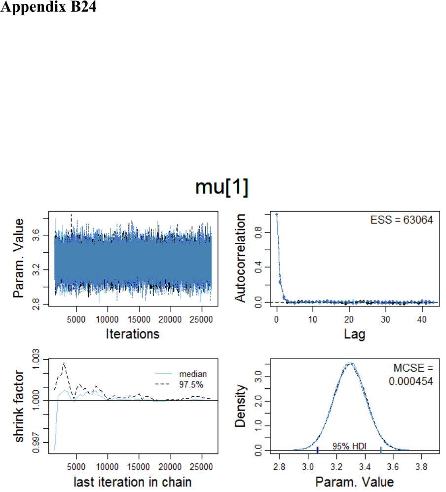
701
Markov Chain convergence diagnostics for
condition V
00
and V
10
This appendix contains the MCMC convergence diagnostic (i.e., ESS and MCSE) for
all parameters. The graphics show the trace plot, autocorrelation plot, shrink factor plot,
and the density plot. All indices indicate that the stationary (equilibrium) distribution π
has been reached.
Figure 113. MCMC diagnostics for μ
1
(experimental condition V
00
).
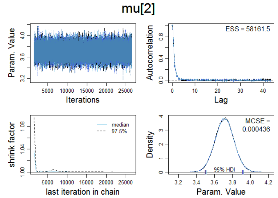
702
Figure 114. MCMC diagnostics for μ
2
(experimental condition V
01
).
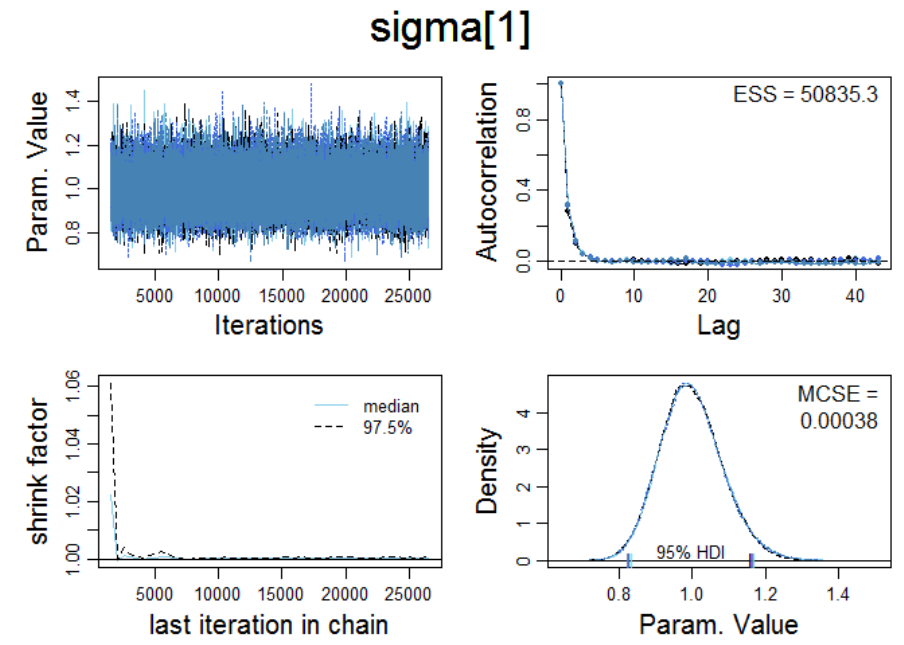
703
Figure 115. MCMC diagnostics for σ
1
(experimental condition V
00
).
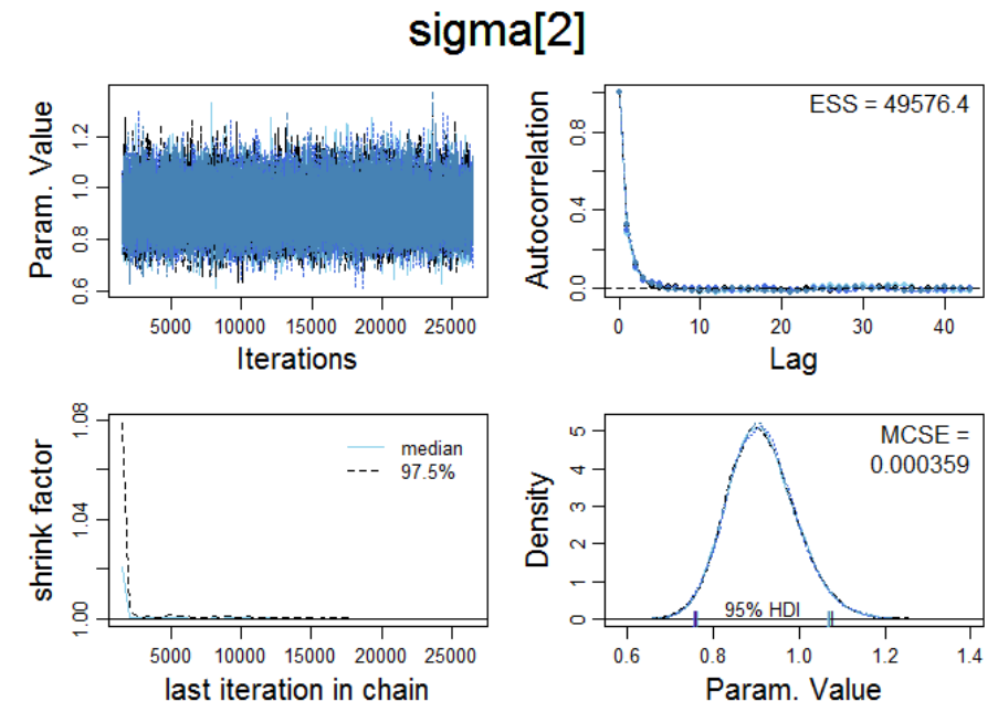
704
Figure 116. MCMC diagnostics for σ
2
(experimental condition V
11
).
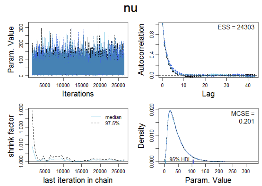
705
Figure 117. MCMC diagnostics for ν.

706
Markov Chain convergence diagnostics for
condition V
00
and V
10
(correlational analysis)
#download data from webserver and import as table
dataexp1 <-
read.table("http://www.irrational-decisions.com/phd-thesis/dataexp1.csv",
header=TRUE, sep=",", na.strings="NA", dec=".",
strip.white=TRUE)
# Model code for the Bayesian alternative to Pearson's correlation test.
# (Bååth, 2014)
require(rjags)
#(Plummer, 2016)
# Setting up the data
x <- dataexp1$v00
y <- dataexp1$v10
xy <- cbind(x, y)
# The model string written in the JAGS language
model_string <- "model {
for(i in 1:n) {
xy[i,1:2] ~ dmt(mu[], prec[ , ], nu)
}
xy_pred[1:2] ~ dmt(mu[], prec[ , ], nu)
# JAGS parameterizes the multivariate t using precision (inverse of
variance)
# rather than variance, therefore here inverting the covariance matrix.

707
prec[1:2,1:2] <- inverse(cov[,])
# Constructing the covariance matrix
cov[1,1] <- sigma[1] * sigma[1]
cov[1,2] <- sigma[1] * sigma[2] * rho
cov[2,1] <- sigma[1] * sigma[2] * rho
cov[2,2] <- sigma[2] * sigma[2]
# Priors
rho ~ dunif(-1, 1)
sigma[1] ~ dunif(sigmaLow, sigmaHigh)
sigma[2] ~ dunif(sigmaLow, sigmaHigh)
mu[1] ~ dnorm(mean_mu, precision_mu)
mu[2] ~ dnorm(mean_mu, precision_mu)
nu <- nuMinusOne+1
nuMinusOne ~ dexp(1/29)
}"
# Initializing the data list and setting parameters for the priors
# that in practice will result in flat priors on mu and sigma.
data_list = list(
xy = xy,
n = length(x),
mean_mu = mean(c(x, y), trim=0.2) ,
precision_mu = 1 / (max(mad(x), mad(y))^2 * 1000000),
sigmaLow = min(mad(x), mad(y)) / 1000 ,
sigmaHigh = max(mad(x), mad(y)) * 1000)
# Initializing parameters to sensible starting values helps the convergence

708
# of the MCMC sampling. Here using robust estimates of the mean (trimmed)
# and standard deviation (MAD).
inits_list = list(mu=c(mean(x, trim=0.2), mean(y, trim=0.2)), rho=cor(x, y,
method="spearman"),
sigma = c(mad(x), mad(y)), nuMinusOne = 5)
# The parameters to monitor.
params <- c("rho", "mu", "sigma", "nu", "xy_pred")
# Running the model
model <- jags.model(textConnection(model_string), data = data_list,
inits = inits_list, n.chains = 3, n.adapt=1000)
update(model, 500) # Burning some samples to the MCMC gods....
samples <- coda.samples(model, params, n.iter=5000)
# Inspecting the posterior
plot(samples)
summary(samples)

709
Iterations = 601:33934
Thinning interval = 1
Number of chains = 3
Sample size per chain = 33334
Diagnostic measures
mean sd mcmc_se n_eff Rhat
rho 0.173 0.110 0.000 54356 1
mu[1] 3.296 0.114 0.000 59397 1
mu[2] 3.717 0.106 0.000 57123 1
sigma[1] 1.004 0.086 0.000 48072 1
sigma[2] 0.920 0.080 0.000 46507 1
nu 43.528 30.588 0.199 23635 1
xy_pred[1] 3.295 1.057 0.003 100001 1
xy_pred[2] 3.716 0.969 0.003 100002 1

710
mcmc_se: estimated standard error of the MCMC approximation of the mea
n
n_eff: a crude measure of effective MCMC sample size.
Rhat: the potential scale reduction factor (at convergence, Rhat=1).
Model parameters
rho: the correlation between dataexp1$v00 and dataexp1$v10
mu[1]: the mean of dataexp1$v00
sigma[1]: the scale of dataexp1$v00,
a consistent estimate of SD when nu is large.
mu[2]: the mean of dataexp1$v10
sigma[2]: the scale of dataexp1$v10
nu: the degrees-of-freedom for the bivariate t distribution
xy_pred[1]: the posterior predictive distribution of dataexp1$v00
xy_pred[2]: the posterior predictive distribution of dataexp1$v10
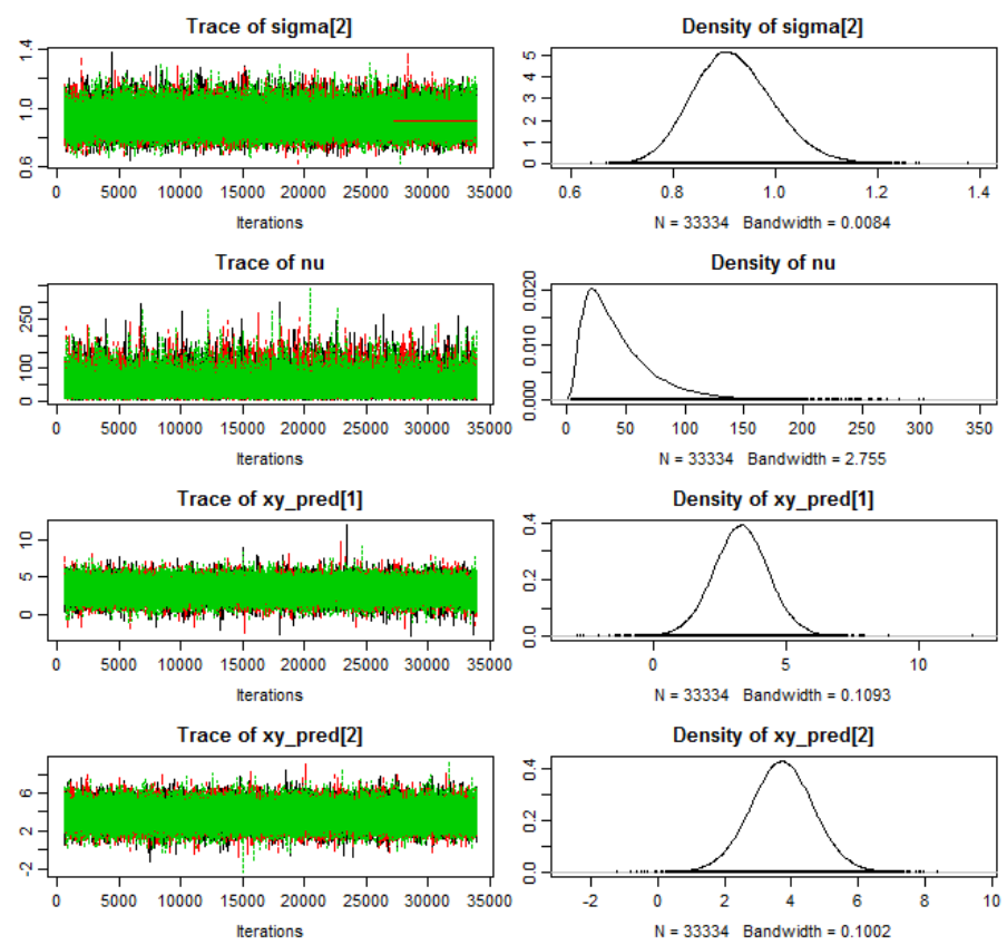
711

712
Measures
mean sd HDIlo HDIup %<comp %>comp
rho 0.173 0.110 -0.044 0.388 0.062 0.938
mu[1] 3.296 0.114 3.073 3.520 0.000 1.000
mu[2] 3.717 0.106 3.509 3.925 0.000 1.000
sigma[1] 1.004 0.086 0.842 1.178 0.000 1.000
sigma[2] 0.920 0.080 0.771 1.082 0.000 1.000
nu 43.528 30.588 5.073 104.975 0.000 1.000
xy_pred[1] 3.295 1.057 1.200 5.380 0.002 0.998
xy_pred[2] 3.716 0.969 1.755 5.592 0.000 1.000
'HDIlo' and 'HDIup' are the limits of a 95% HDI credible interval.
'%<comp' and '%>comp' are the probabilities of the respective paramete
r being
smaller or larger than 0.
Quantiles
q2.5% q25% median q75% q97.5%
rho -0.049 0.099 0.175 0.249 0.384
mu[1] 3.071 3.219 3.296 3.373 3.519
mu[2] 3.509 3.646 3.717 3.787 3.925
sigma[1] 0.849 0.944 1.000 1.059 1.187
sigma[2] 0.776 0.865 0.916 0.971 1.089
nu 9.031 21.705 35.325 56.535 123.410
xy_pred[1] 1.206 2.605 3.297 3.986 5.388
xy_pred[2] 1.791 3.084 3.716 4.351 5.637

713
Markov Chain convergence diagnostics for
condition V
10
and V
11
(correlational analysis)
# Model code for the Bayesian alternative to Pearson's correlation test.
# (Bååth, 2014)
require(rjags)
#(Plummer, 2016)
#download data from webserver and import as table
dataexp1 <-
read.table("http://www.irrational-decisions.com/phd-thesis/dataexp1.csv",
header=TRUE, sep=",", na.strings="NA", dec=".",
strip.white=TRUE)
# Setting up the data
x <- dataexp1$v01
y <- dataexp1$v11
xy <- cbind(x, y)
# The model string written in the JAGS language
model_string <- "model {
for(i in 1:n) {
xy[i,1:2] ~ dmt(mu[], prec[ , ], nu)
}
xy_pred[1:2] ~ dmt(mu[], prec[ , ], nu)
# JAGS parameterizes the multivariate t using precision (inverse of
variance)
# rather than variance, therefore here inverting the covariance matrix.

714
prec[1:2,1:2] <- inverse(cov[,])
# Constructing the covariance matrix
cov[1,1] <- sigma[1] * sigma[1]
cov[1,2] <- sigma[1] * sigma[2] * rho
cov[2,1] <- sigma[1] * sigma[2] * rho
cov[2,2] <- sigma[2] * sigma[2]
# Priors
rho ~ dunif(-1, 1)
sigma[1] ~ dunif(sigmaLow, sigmaHigh)
sigma[2] ~ dunif(sigmaLow, sigmaHigh)
mu[1] ~ dnorm(mean_mu, precision_mu)
mu[2] ~ dnorm(mean_mu, precision_mu)
nu <- nuMinusOne+1
nuMinusOne ~ dexp(1/29)
}"
# Initializing the data list and setting parameters for the priors
# that in practice will result in flat priors on mu and sigma.
data_list = list(
xy = xy,
n = length(x),
mean_mu = mean(c(x, y), trim=0.2) ,
precision_mu = 1 / (max(mad(x), mad(y))^2 * 1000000),
sigmaLow = min(mad(x), mad(y)) / 1000 ,
sigmaHigh = max(mad(x), mad(y)) * 1000)
# Initializing parameters to sensible starting values helps the convergence

715
# of the MCMC sampling. Here using robust estimates of the mean (trimmed)
# and standard deviation (MAD).
inits_list = list(mu=c(mean(x, trim=0.2), mean(y, trim=0.2)), rho=cor(x, y,
method="spearman"),
sigma = c(mad(x), mad(y)), nuMinusOne = 5)
# The parameters to monitor.
params <- c("rho", "mu", "sigma", "nu", "xy_pred")
# Running the model
model <- jags.model(textConnection(model_string), data = data_list,
inits = inits_list, n.chains = 3, n.adapt=1000)
update(model, 500) # Burning some samples to the MCMC gods....
samples <- coda.samples(model, params, n.iter=5000)
# Inspecting the posterior
plot(samples)
summary(samples)

716
Iterations = 601:33934
Thinning interval = 1
Number of chains = 3
Sample size per chain = 33334
Diagnostic measures
mean sd mcmc_se n_eff Rhat
rho 0.198 0.109 0.000 57872 1.000
mu[1] 7.218 0.127 0.001 54686 1.000
mu[2] 6.685 0.120 0.001 55458 1.000
sigma[1] 1.102 0.100 0.001 40148 1.000
sigma[2] 1.045 0.095 0.000 41779 1.000
nu 34.731 27.521 0.207 17853 1.001
xy_pred[1] 7.215 1.175 0.004 100001 1.000
xy_pred[2] 6.686 1.113 0.004 99369 1.000

717
mcmc_se: estimated standard error of the MCMC approximation of the mea
n.
n_eff: a crude measure of effective MCMC sample size.
Rhat: the potential scale reduction factor (at convergence, Rhat=1).
Model parameters
rho: the correlation between dataexp1$v01 and dataexp1$v11
mu[1]: the mean of dataexp1$v01
sigma[1]: the scale of dataexp1$v01 , a consistent
estimate of SD when nu is large.
mu[2]: the mean of dataexp1$v11
sigma[2]: the scale of dataexp1$v11
nu: the degrees-of-freedom for the bivariate t distribution
xy_pred[1]: the posterior predictive distribution of dataexp1$v01
xy_pred[2]: the posterior predictive distribution of dataexp1$v11
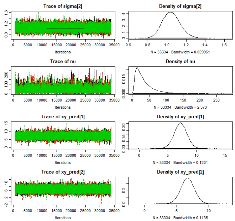
718

719
Measures
mean sd HDIlo HDIup %<comp %>comp
rho 0.198 0.109 -0.017 0.409 0.038 0.962
mu[1] 7.218 0.127 6.966 7.464 0.000 1.000
mu[2] 6.685 0.120 6.447 6.921 0.000 1.000
sigma[1] 1.102 0.100 0.909 1.304 0.000 1.000
sigma[2] 1.045 0.095 0.861 1.232 0.000 1.000
nu 34.731 27.521 3.500 90.205 0.000 1.000
xy_pred[1] 7.215 1.175 4.917 9.561 0.000 1.000
xy_pred[2] 6.686 1.113 4.473 8.875 0.000 1.000
'HDIlo' and 'HDIup' are the limits of a 95% HDI credible interval.
'%<comp' and '%>comp' are the probabilities of the respective parameter being
smaller or larger than 0.
Quantiles
q2.5% q25% median q75% q97.5%
rho -0.021 0.124 0.200 0.273 0.405
mu[1] 6.969 7.133 7.218 7.303 7.467
mu[2] 6.448 6.605 6.685 6.765 6.922
sigma[1] 0.916 1.034 1.098 1.166 1.313
sigma[2] 0.870 0.980 1.042 1.106 1.244
nu 6.467 15.385 26.501 45.377 108.995
xy_pred[1] 4.891 6.456 7.209 7.974 9.542
xy_pred[2] 4.489 5.965 6.684 7.400 8.895
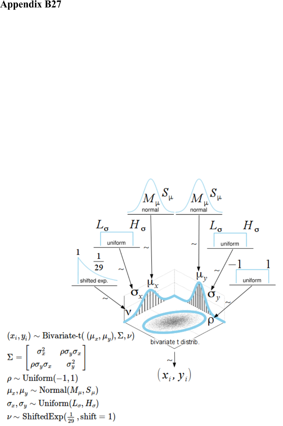
720
Correlational analysis
Next, we investigate the bivariate correlations between experimental conditions. The
Pearson's product-moment correlation coefficient for experimental condition V
00
vs. V
01
was statistically nonsignificant, r = 0.097, p = 0.388, 95% CI [-0.31, 0.12]. Ergo, this
frequentist analysis indicated that H
0
cannot be rejected (i.e., the correlation is equal to
zero). In addition, we computed the Bayesian equivalent of Pearson's correlation test
using R and JAGS (Bååth, 2014). We defined the same noncommittal broad priors as in
the previous analysis. The associated hierarchical Bayesian model is illustrated in
Figure 118.

721
Figure 118. Pictogram of the Bayesian hierarchical model for the correlational analysis
(Friendly et al., 2013). The underlying JAGS-model can be downloaded from the
following URL: http://irrational-decisions.com/?page_id=2370
We performed the simulation with 1000 adaptations, 500 burn-in steps, and 10000
iterations (no thinning interval, 3 chains in parallel, sample size per chain = 33334). The
convergence diagnostics indicated that the equilibrium distribution π had been reached.
Various diagnostic measures are printed in

722
Table 51
Summary of convergence diagnostics for ρ, μ
1
, μ
2
, σ
1
, σ
2
, ν, and the posterior predictive
distribution of V
00
and V
10
.
Diagnostic measures
mean sd mcmc_se n_eff Rhat
rho 0.173 0.110 0.000 54356 1
mu[1] 3.296 0.114 0.000 59397 1
mu[2] 3.717 0.106 0.000 57123 1
sigma[1] 1.004 0.086 0.000 48072 1
sigma[2] 0.920 0.080 0.000 46507 1
nu 43.528 30.588 0.199 23635 1
xy_pred[1] 3.295 1.057 0.003 100001 1
xy_pred[2] 3.716 0.969 0.003 100002 1
Model parameters:
• ρ (rho): The correlation between experimental condition V
00
and V
10
• μ
1
(mu[1]): The mean of V
00
• σ
1
(sigma[1]): The scale of V
00
, a consistent estimate of SD when nu is large.
• μ
2
(mu[2]): the mean of V
10
• σ
1
(sigma[2]): the scale of V
10
• ν (nu): The degrees-of-freedom for the bivariate t distribution
• xy_pred[1]: The posterior predictive distribution of V
00
• xy_pred[2]: The posterior predictive distribution of V
10
Convergence diagnostics:
• mcmc_se: The estimated standard error of the MCMC approximation of the
mean.
• n_eff: A crude measure of effective MCMC sample size.

723
• Rhat: the potential scale reduction factor (at convergence, Rhat=1).
The results of the Bayesian MCMC analysis indicated that the estimated correlation
between condition V
00
vs. V
01
was ρ = 0.17 and the associated 95% Bayesian posterior
high density credible interval ranged from [-0.05, 0.38]. Furthermore, it can be
concluded that the correlation between condition V
00
vs. V
01
is > 0 by a probability of
0.934 (and < 0 by a probability of 0.066). The results are visualised in Figure 119. A
numerical summary is given in Table 52.
Table 52
Numerical summary for all parameters associated with experimental condition V
10
and
V
01
and their corresponding 95% posterior high density credible intervals.
Measures
mean sd HDIlo HDIup %<comp %>comp
rho 0.173 0.110 -0.044 0.388 0.062 0.938
mu[1] 3.296 0.114 3.073 3.520 0.000 1.000
mu[2] 3.717 0.106 3.509 3.925 0.000 1.000
sigma[1] 1.004 0.086 0.842 1.178 0.000 1.000
sigma[2] 0.920 0.080 0.771 1.082 0.000 1.000
nu 43.528 30.588 5.073 104.975 0.000 1.000
xy_pred[1] 3.295 1.057 1.200 5.380 0.002 0.998
xy_pred[2] 3.716 0.969 1.755 5.592 0.000 1.000
Note. 'HDIlo' and 'HDIup' are the limits of a 95% HDI credible interval.
'%<comp' and '%>comp' are the probabilities of the respective parameter being smaller
or larger than 0.
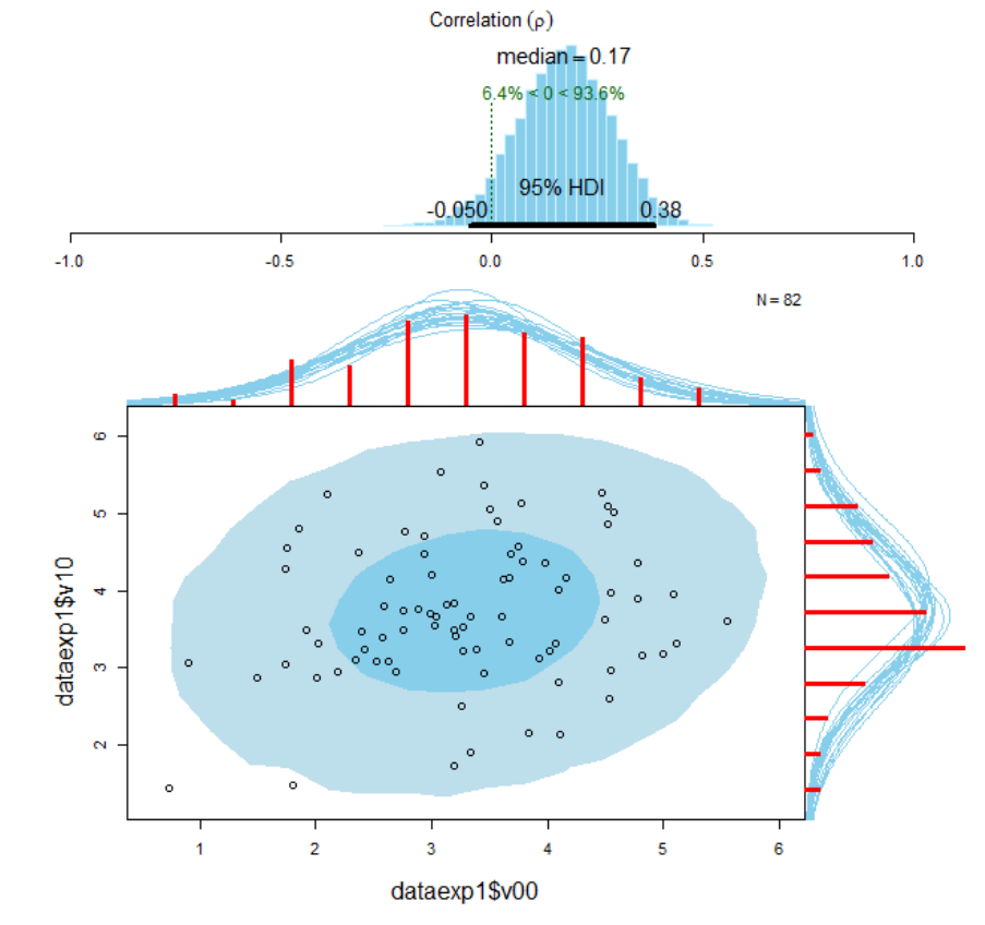
724
Figure 119. Visualisation of the results of the Bayesian correlational analysis for
experimental condition V
00
and V
01
with associated posterior high density credible
intervals and marginal posterior predictive plots.
This upper panel of the plot displays the posterior distribution for the correlation ρ (rho)
with its associated 95% HDI. In addition, the lower panel of the plot shows the original
empirical data with superimposed posterior predictive distributions. The posteriors
predictive distributions allow to predict new data and can also be utilised to assess the
model fit. It can be seen that the model fits the data reasonably well. The two
histograms (in red) visualise the marginal distributions of the experimental data. The

725
dark-blue ellipse encompasses the 50% highest density region and the light-blue ellipse
spans the 95% high density region, thereby providing intuitive visual insights into the
probabilistic distribution of the data (Friendly et al., 2013; Hollowood, 2016). The
Bayesian analysis provides much more detailed and precise information compared to
the classical frequentist Pearsonian approach.
We repeated the same analysis for experimental condition V
10
and V
11
. Pearson’s r was
again nonsignificant, r = 0.02, p = 0.86, 95% CI [-0.20, 0.24], indicating that the
correlation between experimental conditions V
10
and V
11
is statistically non-significant,
i.e., H
0
cannot be rejected. The estimated Bayesian correlation was ρ = 0.20, 95% HDI
[-0.03, 0.41]. The analysis indicated that the correlation between condition V
00
vs. V
01
is > 0 by a probability of 0.958 (and < 0 by a probability of 0.042). A visual summary of
the results is provided in Figure 129 and provided a quantitative overview of the results.
Table 53
Numerical summary for all parameters associated with experimental condition V
01
and
V
11
and their corresponding 95% posterior high density credible intervals.
Measures
mean sd HDIlo HDIup %<comp %>comp
rho 0.198 0.109 -0.017 0.409 0.038 0.962
mu[1] 7.218 0.127 6.966 7.464 0.000 1.000
mu[2] 6.685 0.120 6.447 6.921 0.000 1.000
sigma[1] 1.102 0.100 0.909 1.304 0.000 1.000
sigma[2] 1.045 0.095 0.861 1.232 0.000 1.000
nu 34.731 27.521 3.500 90.205 0.000 1.000
xy_pred[1] 7.215 1.175 4.917 9.561 0.000 1.000
xy_pred[2] 6.686 1.113 4.473 8.875 0.000 1.000
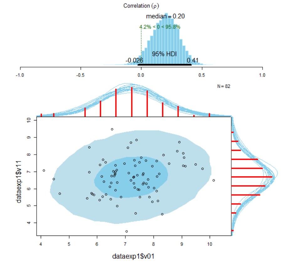
726
Figure 120. Visualisation of the results of the Bayesian correlational analysis for
experimental condition V
10
and V
11
with associated posterior high density credible
intervals and marginal posterior predictive plots.
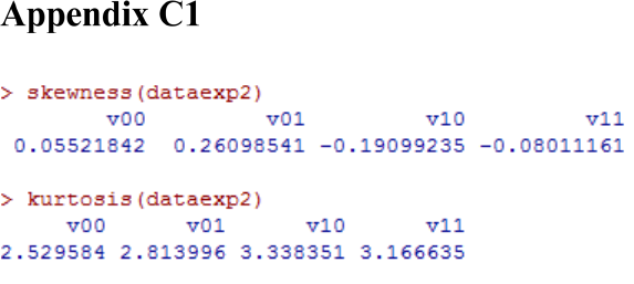
727
Appendix C Experiment 2
Skewness and kurtosis

728
Anscombe-Glynn kurtosis tests
(Anscombe & Glynn, 1983)
data: dataexp2$v00
kurt = 2.52960, z = -0.65085, p-value = 0.5151
alternative hypothesis: kurtosis is not equal to 3
data: dataexp2$v01
kurt = 2.81400, z = 0.02739, p-value = 0.9781
alternative hypothesis: kurtosis is not equal to 3
data: dataexp2$v10
kurt = 3.33840, z = 0.92903, p-value = 0.3529
alternative hypothesis: kurtosis is not equal to 3
data: dataexp2$v11
kurt = 3.16660, z = 0.67032, p-value = 0.5027
alternative hypothesis: kurtosis is not equal to 3
D'Agostino skewness tests (D’Agostino, 1970)
data: dataexp2$v00
skew = 0.055198, z = 0.194460, p-value = 0.8458
alternative hypothesis: data have a skewness
data: dataexp2$v01
skew = 0.26100, z = 0.90906, p-value = 0.3633
alternative hypothesis: data have a skewness
data: dataexp2$v10
skew = -0.19101, z = -0.66895, p-value = 0.5035
alternative hypothesis: data have a skewness
data: dataexp2$v11
729
skew = -0.080075, z = -0.281940, p-value = 0.778
alternative hypothesis: data have a skewness
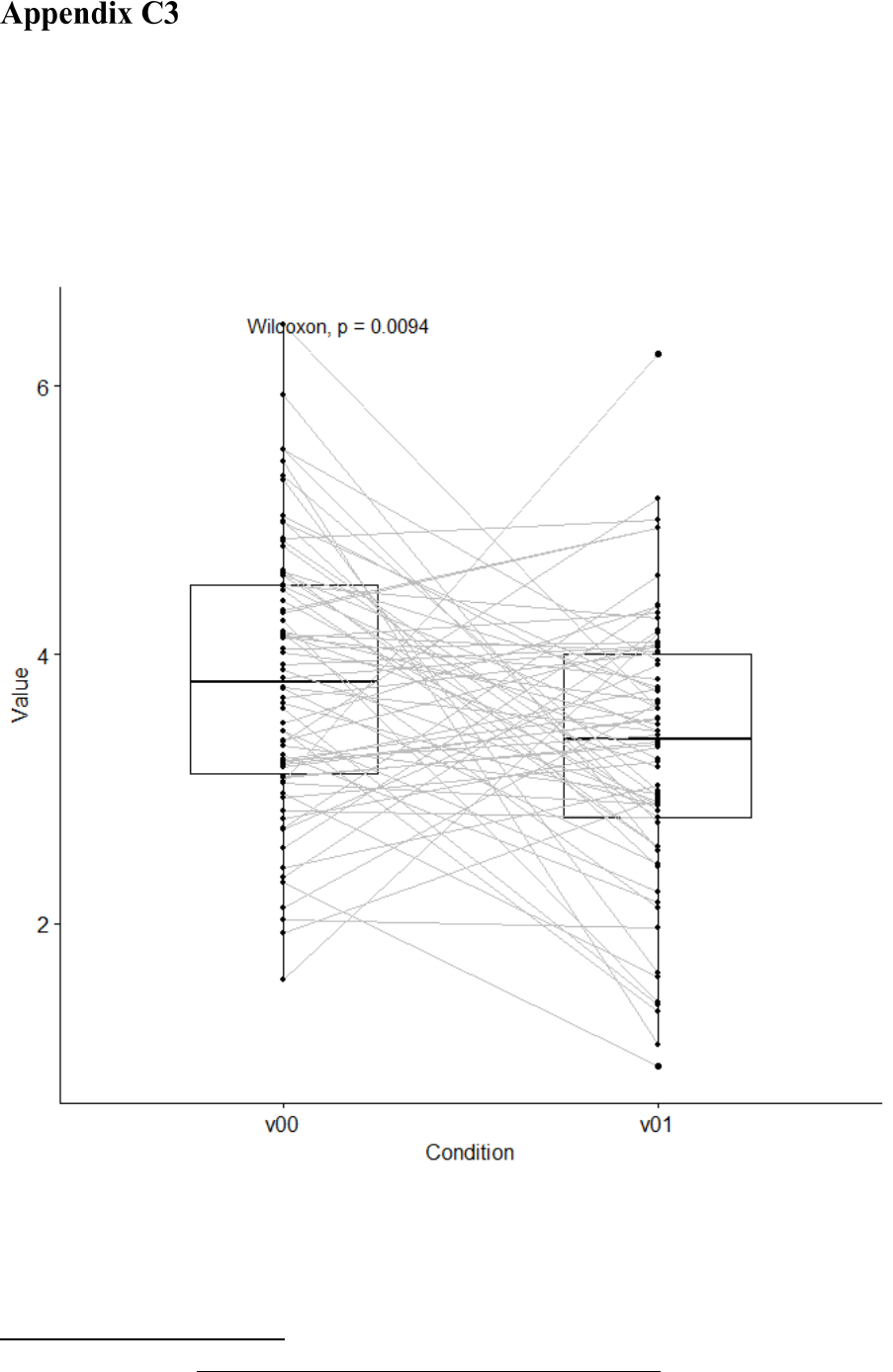
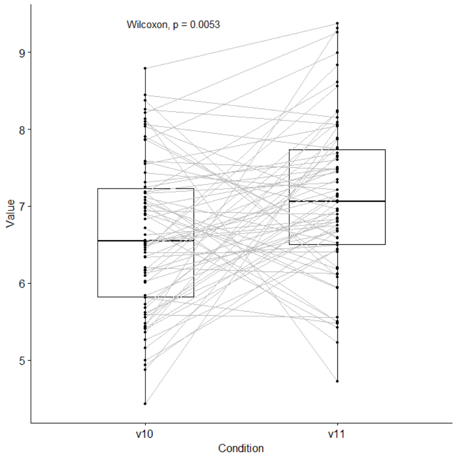
731
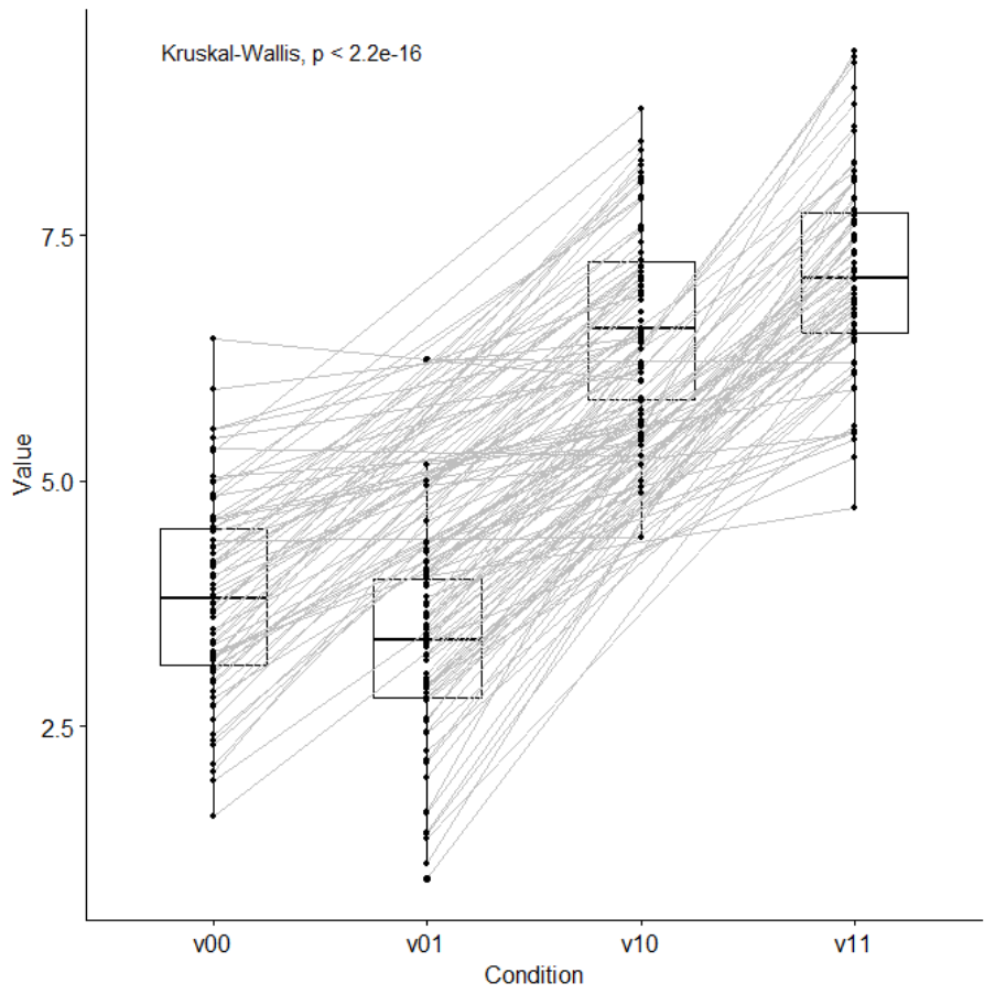
732

733
MCMC convergence diagnostics for
experimental condition V
00
vs. V
01
This appendix contains the MCMC convergence diagnostic (i.e., MCSE, ESS, Rhat) for
all parameters. The associated graphics show the trace plot and the density plot.
Iterations = 601:33934
Thinning interval = 1
Number of chains = 3
Sample size per chain = 33334
Diagnostic measures
mean sd mcmc_se n_eff Rhat
mu_diff 0.523 0.183 0.001 61589 1
sigma_diff 1.467 0.143 0.001 45052 1
nu 37.892 30.417 0.216 19809 1
eff_size 0.360 0.129 0.001 61073 1
diff_pred 0.533 1.571 0.005 100001 1
Model parameters:
• μ
∆
(mu_diff): The mean pairwise difference between experimental conditions
• σ
∆
(sigma_diff): the scale of the pairwise difference (a consistent estimate of SD
when nu is large)
• ν (nu): The degrees-of-freedom for the bivariate t distribution fitted to the
pairwise difference
• δ (eff_size): the effect size calculated as (
0)/
.
• μ
∆pred
(diff_pred): predicted distribution for a new datapoint generated as the
pairwise difference between experimental conditions
734
Convergence diagnostics:
• mcmc_se (Monte Carlo Standard Error, MCSE): The estimated standard error of
the MCMC approximation of the mean.
• n_eff (Effective Sample Size, ESS): A crude measure of effective MCMC
sample size.
• Rhat (Shrink factor,
): the potential scale reduction factor (at convergence,
1).
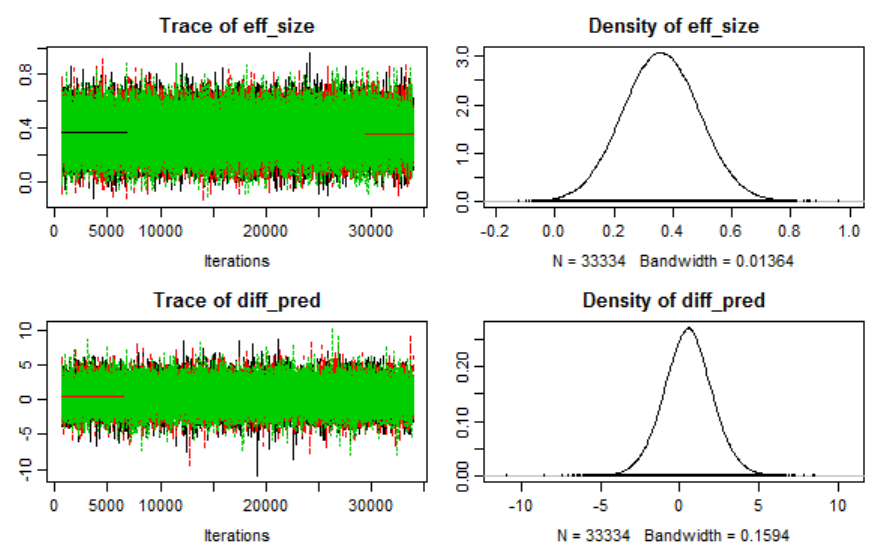
735
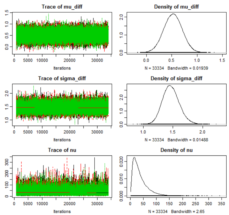
736

737
MCMC convergence diagnostics for
xperimental condition V
10
vs V
11
Iterations = 601:33934
Thinning interval = 1
Number of chains = 3
Sample size per chain = 33334
Diagnostic measures
mean sd mcmc_se n_eff Rhat
mu_diff -0.485 0.171 0.001 60590 1
sigma_diff 1.358 0.137 0.001 42080 1
nu 35.134 28.790 0.206 19744 1
eff_size -0.361 0.131 0.001 59362 1
diff_pred -0.485 1.461 0.005 100001 1
Model parameters:
• μ
∆
(mu_diff): The mean pairwise difference between experimental conditions
• σ
∆
(sigma_diff): the scale of the pairwise difference (a consistent estimate of SD
when nu is large)
• ν (nu): The degrees-of-freedom for the bivariate t distribution fitted to the
pairwise difference
• δ (eff_size): the effect size calculated as (
0)/
.
• μ
∆pred
(diff_pred): predicted distribution for a new datapoint generated as the
pairwise difference between experimental conditions
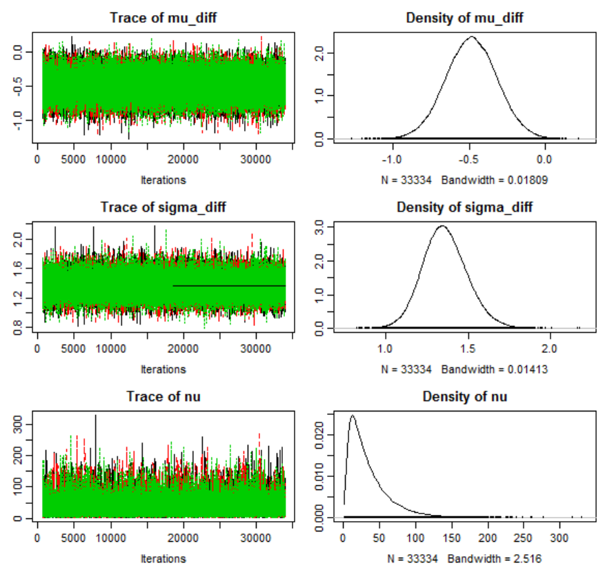
738

739

740
Visualisation of MCMC: 3-dimensional
scatterplot with associated concentration eclipse
“I know of no person or group that is taking nearly adequate advantage of the graphical
potentialities of the computer.”
~ John Tukey
R is equipped with a powerful computer graphic system which can be extended with
additional libraries, e.g., OpenGL (Open Graphics Library; Hearn & Baker, 2004;
Murdoch, 2001). The following three-dimensional visualisations was created with the
R package “scatterplot3d” (Ligges & Mächler, 2003) which utilises Open GL. The
graphic depicts the relationship between experimental conditions, i.e., V
00
versus V
01
,
based on 1200 steps extracted from the MCMC samples. An interactive fullscreen-
version which allows closer inspection of the data is available under the following URL:
http://irrational-decisions.com/phd-thesis/scatterplot3d-openGL.mp4
The MCMC dataset and the R code are also available online: http://irrational-
decisions.com/?page_id=2100

741
Figure 121. 3D scatterplot of the MCMC dataset with 50% concentration ellipsoid
visualising the relation between μ
1
(V
00
) and μ
2
(V
01
), and v in 3-dimensional parameter
space.
Ellipsoids are an intuitive way to understanding of multivariate relationships (Kruschke,
2014). Ellipsoids provide a visual summary for the means, the standard deviations, and
correlations in 3-dimensional data space (Friendly et al., 2013).
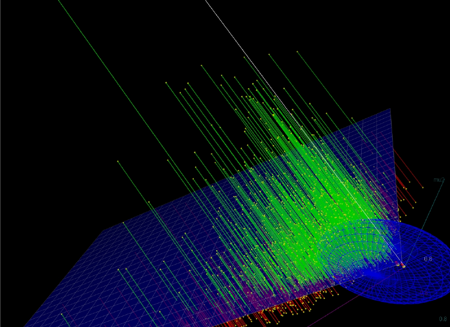
742
Figure 122. 3D scatterplot (with regression plane) of MCMC dataset with increased
zoom-factor in order to emphasize the concentration of the values of θ.

743
mcmcExp2 <- readXL("C:/Users/cgermann/Documents/BEST/mcmc-exp2.xlsx",
rownames=FALSE, header=TRUE, na="", sheet="mcmc-chain-exp2-with-header",
stringsAsFactors=TRUE)
library(rgl, pos=14)
library(nlme, pos=15)
library(mgcv, pos=15)
scatter3d(v~mu1+mu2, data=mcmcExp2, surface=TRUE, bg="black", axis.scales=TRUE,
grid=TRUE, ellipsoid=TRUE, model.summary=TRUE)
Code 9. R commander code for 3D scatterplot with concertation ellipsoid.
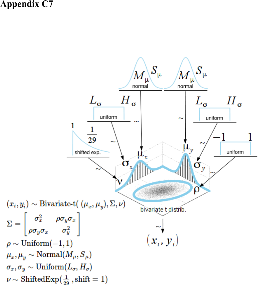
744
Correlational analysis
Appendix C7.1 Hierarchical Bayesian model
The associated hierarchical Bayesian model is described in greater detail in the analysis
section of Experiment 1.

745
Appendix C7.2 Convergence diagnostics for the Bayesian
correlational analysis (V
10
vs. V
11
)
Iterations = 601:33934
Thinning interval = 1
Number of chains = 3
Sample size per chain = 33334
Diagnostic measures
mean sd mcmc_se n_eff Rhat
rho -0.079 0.122 0.001 58760 1.000
mu[1] 3.819 0.126 0.001 58238 1.000
mu[2] 3.298 0.125 0.001 60951 1.000
sigma[1] 1.017 0.096 0.000 48272 1.000
sigma[2] 1.005 0.097 0.000 46355 1.000
nu 39.910 29.999 0.210 21090 1.001
xy_pred[1] 3.817 1.071 0.003 100002 1.000
xy_pred[2] 3.301 1.064 0.003 98680 1.000
Model parameters:
• ρ (rho): The correlation between experimental condition V
00
and V
10
• μ
1
(mu[1]): The mean of V
00
• σ
1
(sigma[1]): The scale of V
00
, a consistent estimate of SD when nu is large.
• μ
2
(mu[2]): the mean of V
10
• σ
1
(sigma[2]): the scale of V
10
• ν (nu): The degrees-of-freedom for the bivariate t distribution
• xy_pred[1]: The posterior predictive distribution of V
00
• xy_pred[2]: The posterior predictive distribution of V
10
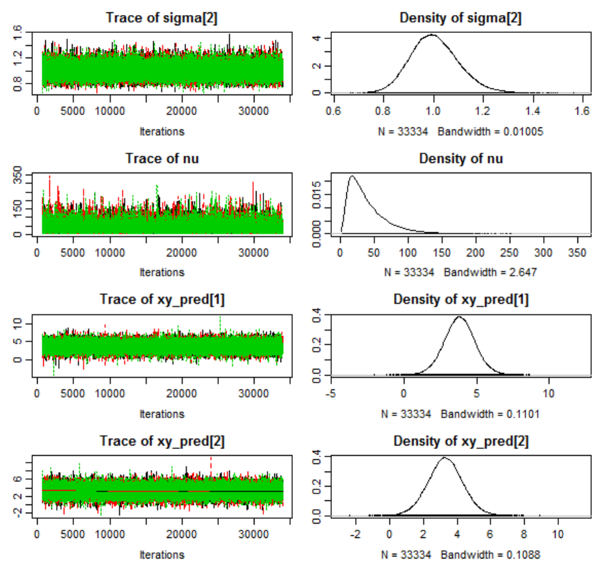
746
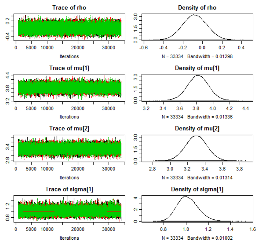
747

748
Appendix C7.3 Convergence diagnostics for the Bayesian
correlational analysis (V
10
and V
11
)
Iterations = 601:33934
Thinning interval = 1
Number of chains = 3
Sample size per chain = 33334
Diagnostic measures
mean sd mcmc_se n_eff Rhat
rho 0.034 0.124 0.001 61483 1
mu[1] 6.617 0.126 0.001 61561 1
mu[2] 7.098 0.124 0.000 61224 1
sigma[1] 1.009 0.094 0.000 49525 1
sigma[2] 0.999 0.095 0.000 47846 1
nu 42.025 30.704 0.211 21292 1
xy_pred[1] 6.619 1.069 0.003 99485 1
xy_pred[2] 7.101 1.054 0.003 97846 1
Model parameters:
• ρ (rho): The correlation between experimental condition V
00
and V
10
• μ
1
(mu[1]): The mean of V
00
• σ
1
(sigma[1]): The scale of V
00
, a consistent estimate of SD when nu is large.
• μ
2
(mu[2]): the mean of V
10
• σ
1
(sigma[2]): the scale of V
10
• ν (nu): The degrees-of-freedom for the bivariate t distribution
• xy_pred[1]: The posterior predictive distribution of V
00
• xy_pred[2]: The posterior predictive distribution of V
10
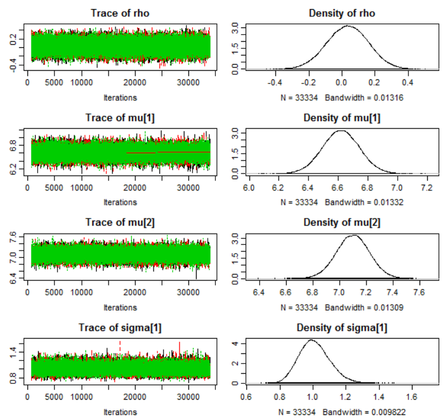
749
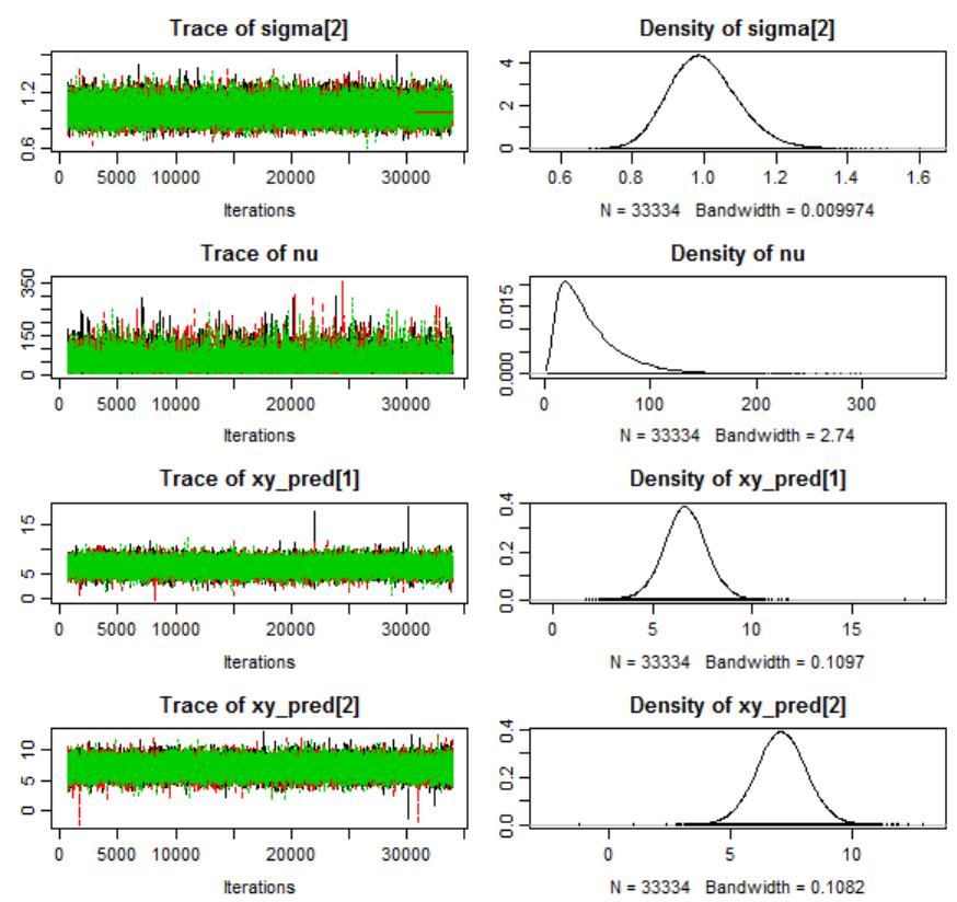
750

751
Appendix C7.4 Pearson's product-moment correlation
between experimental condition V00 vs. V10
Pearson's product-moment correlation
data: v00 and v01
t = -0.65285, df = 68, p-value = 0.5161
alternative hypothesis: true correlation is not equal to 0
95 percent confidence interval:
-0.3081814 0.1590001
sample estimates:
cor
-0.07892249

752
mean sd HDIlo HDIup %<comp %>comp
rho -0.079 0.122 -0.315 0.163 0.740 0.260
mu[1] 3.819 0.126 3.572 4.069 0.000 1.000
mu[2] 3.298 0.125 3.055 3.545 0.000 1.000
sigma[1] 1.017 0.096 0.834 1.209 0.000 1.000
sigma[2] 1.005 0.097 0.821 1.198 0.000 1.000
nu 39.910 29.999 3.967 99.213 0.000 1.000
xy_pred[1] 3.817 1.071 1.678 5.924 0.001 0.999
xy_pred[2] 3.301 1.064 1.176 5.391 0.002 0.998
Model parameters:
• ρ (rho): The correlation between experimental condition V
00
and V
10
• μ
1
(mu[1]): The mean of V
00
• σ
1
(sigma[1]): The scale of V
00
, a consistent estimate of SD when nu is large.
• μ
2
(mu[2]): the mean of V
10
• σ
1
(sigma[2]): the scale of V
10
• ν (nu): The degrees-of-freedom for the bivariate t distribution
• xy_pred[1]: The posterior predictive distribution of V
00
• xy_pred[2]: The posterior predictive distribution of V
10
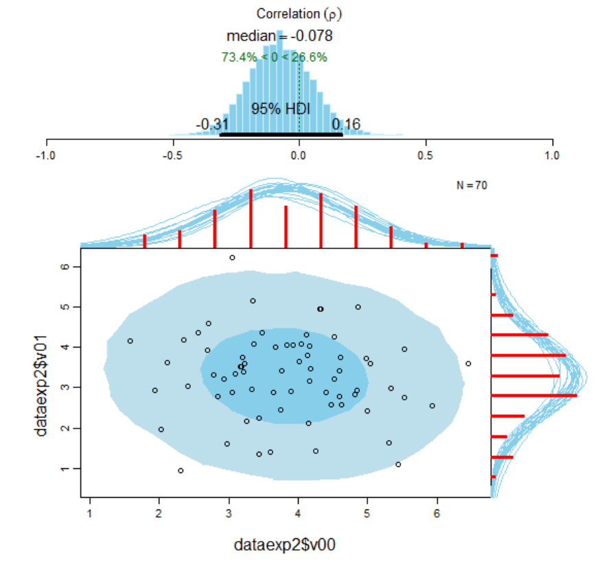
753
Figure 123. Visualisation of the results of the Bayesian correlational analysis for
experimental condition V
00
and V
01
with associated posterior high density credible
intervals and marginal posterior predictive plots.
This upper panel of the plot displays the posterior distribution for the correlation ρ (rho)
with its associated 95% HDI. In addition, the lower panel of the plot shows the original
empirical data with superimposed posterior predictive distributions. The posteriors
predictive distributions allow to predict new data and can also be utilised to assess the
model fit. It can be seen that the model fits the data reasonably well. The two
histograms (in red) visualise the marginal distributions of the experimental data. The
754
dark-blue ellipse encompasses the 50% highest density region and the light-blue ellipse
spans the 95% high density region, thereby providing intuitive visual insights into the
probabilistic distribution of the data (Hollowood, 2016). The Bayesian analysis provides
much more detailed and precise information compared to the classical frequentist
Pearsonian approach.

755
Appendix C7.5 Pearson's product-moment correlations
between experimental conditions V
01
vs V
11
Pearson's product-moment correlation
data: v10 and v11
t = 0.33564, df = 68, p-value = 0.7382
alternative hypothesis: true correlation is not equal to 0
95 percent confidence interval:
-0.1961796 0.2730340
sample estimates:
cor
0.04066911

756
Table 54
Numerical summary for all parameters associated with experimental condition V
10
and
V
01
and their corresponding 95% posterior high density credible intervals.
mean sd HDIlo HDIup %<comp %>comp
rho 0.034 0.124 -0.210 0.275 0.39 0.61
mu[1] 6.617 0.126 6.368 6.863 0.00 1.00
mu[2] 7.098 0.124 6.855 7.341 0.00 1.00
sigma[1] 1.009 0.094 0.831 1.194 0.00 1.00
sigma[2] 0.999 0.095 0.821 1.191 0.00 1.00
nu 42.025 30.704 4.393 102.736 0.00 1.00
xy_pred[1] 6.619 1.069 4.491 8.726 0.00 1.00
xy_pred[2] 7.101 1.054 4.980 9.149 0.00 1.00
Note. 'HDIlo' and 'HDIup' are the limits of a 95% HDI credible interval.
'%<comp' and '%>comp' are the probabilities of the respective parameter being smaller
or larger than 0.
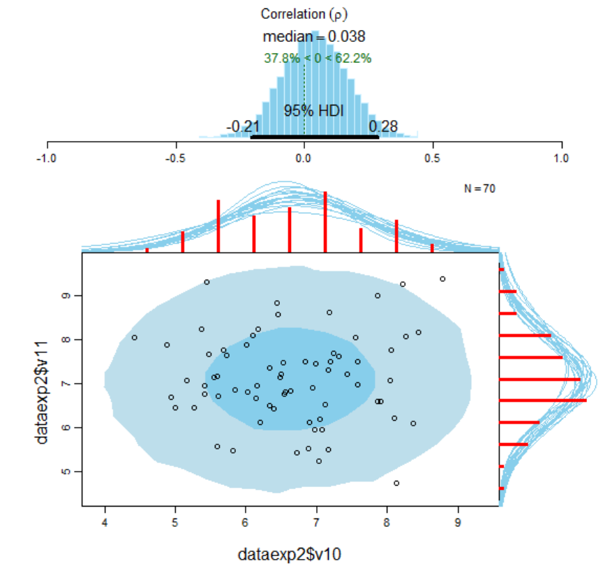
757
Figure 124. Visualisation of the results of the Bayesian correlational analysis for
experimental condition V
10
and V
11
with associated posterior high density credible
intervals and marginal posterior predictive plots.

758
JAGS model code for the correlational
analysis
# Model code for the Bayesian alternative to Pearson's correlation
test.
# (Bååth, 2014)
require(rjags)
#(Plummer, 2016)
#download data from webserver and import as table
Dataexp2 <-
read.table("http://www.irrational-decisions.com/phd-
thesis/dataexp2.csv", header=TRUE, sep=",", na.strings="NA",
dec=".", strip.white=TRUE)
# Setting up the data
x <- dataexp1$v01
y <- dataexp1$v11
xy <- cbind(x, y)
# The model string written in the JAGS language
model_string <- "model {
for(i in 1:n) {
xy[i,1:2] ~ dmt(mu[], prec[ , ], nu)
}
xy_pred[1:2] ~ dmt(mu[], prec[ , ], nu)

759
# JAGS parameterizes the multivariate t using precision (inverse
of variance)
# rather than variance, therefore here inverting the covariance
matrix.
prec[1:2,1:2] <- inverse(cov[,])
# Constructing the covariance matrix
cov[1,1] <- sigma[1] * sigma[1]
cov[1,2] <- sigma[1] * sigma[2] * rho
cov[2,1] <- sigma[1] * sigma[2] * rho
cov[2,2] <- sigma[2] * sigma[2]
# Priors
rho ~ dunif(-1, 1)
sigma[1] ~ dunif(sigmaLow, sigmaHigh)
sigma[2] ~ dunif(sigmaLow, sigmaHigh)
mu[1] ~ dnorm(mean_mu, precision_mu)
mu[2] ~ dnorm(mean_mu, precision_mu)
nu <- nuMinusOne+1
nuMinusOne ~ dexp(1/29)
}"
# Initializing the data list and setting parameters for the priors
# that in practice will result in flat priors on mu and sigma.
data_list = list(
xy = xy,
n = length(x),

760
mean_mu = mean(c(x, y), trim=0.2) ,
precision_mu = 1 / (max(mad(x), mad(y))^2 * 1000000),
sigmaLow = min(mad(x), mad(y)) / 1000 ,
sigmaHigh = max(mad(x), mad(y)) * 1000)
# Initializing parameters to sensible starting values helps the
convergence
# of the MCMC sampling. Here using robust estimates of the mean
(trimmed)
# and standard deviation (MAD).
inits_list = list(mu=c(mean(x, trim=0.2), mean(y, trim=0.2)),
rho=cor(x, y, method="spearman"),
sigma = c(mad(x), mad(y)), nuMinusOne = 5)
# The parameters to monitor.
params <- c("rho", "mu", "sigma", "nu", "xy_pred")
# Running the model
model <- jags.model(textConnection(model_string), data = data_list,
inits = inits_list, n.chains = 3, n.adapt=1000)
update(model, 500)
samples <- coda.samples(model, params, n.iter=5000)
# Inspecting the posterior
plot(samples)
summary(samples)
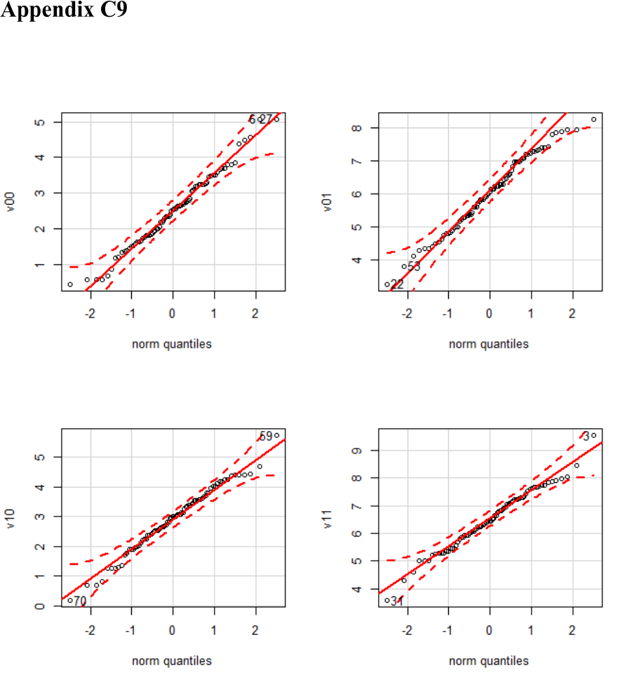
761
Tests of Gaussianity
Figure 125. Q-Q plots for visual inspection of distribution characteristics.
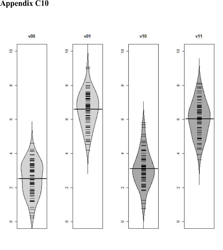
762
Symmetric beanplots for direct visual
comparison between experimental conditions
Figure 126. Symmetric beanplots for visual inspection of distribution characteristics.
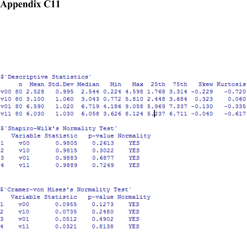
763
Descriptive statistics and various normality
tests
Table 55
Descriptive statistics and various normality tests.
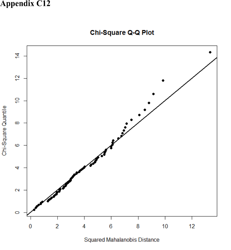
764
χ2 Q-Q plot (Mahalanobis Distance)
Figure 127. χ2 Q-Q plot (Mahalanobis Distance, D
2
).
Note: Q-Q plot based on Royston's Multivariate Normality Test (see next page).
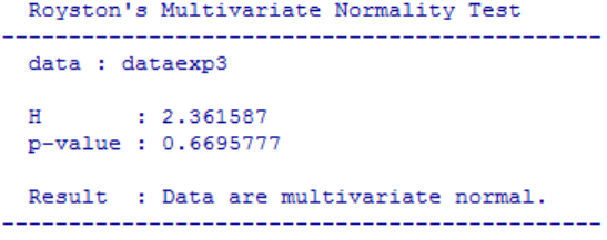
765
Table 56
Royston’s multivariate normality test.
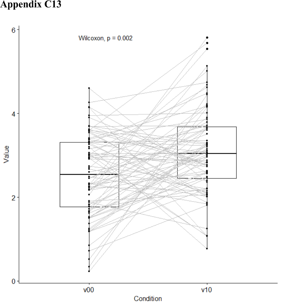
766
Connected boxplots (with Wilcoxon test)
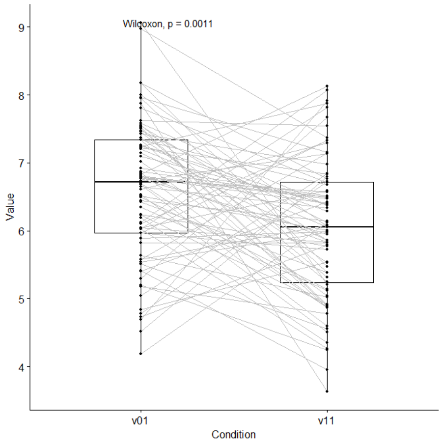
767
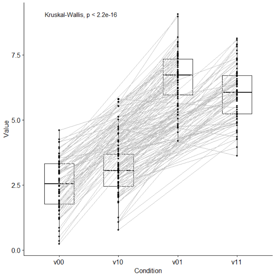
768

769
Correlational analysis
1
st
pair
Pearson's product-moment correlation
data: v00 and v10
t = 1.7026, df = 80, p-value = 0.09253
alternative hypothesis: true correlation is not equal to 0
95 percent confidence interval:
-0.03128247 0.38824652
sample estimates:
cor
0.1869941

770
Table 57
Numerical summary for all parameters associated with experimental condition V
10
and
V
01
and their corresponding 95% posterior high density credible intervals.
Measures
mean sd HDIlo HDIup %<comp %>comp
rho -0.080 0.114 -0.301 0.143 0.761 0.239
mu[1] 2.531 0.115 2.306 2.757 0.000 1.000
mu[2] 3.088 0.121 2.853 3.328 0.000 1.000
sigma[1] 0.999 0.085 0.836 1.167 0.000 1.000
sigma[2] 1.052 0.093 0.876 1.236 0.000 1.000
nu 46.710 31.655 5.671 109.173 0.000 1.000
xy_pred[1] 2.526 1.042 0.460 4.554 0.009 0.991
xy_pred[2] 3.087 1.103 0.882 5.254 0.004 0.996
Note. 'HDIlo' and 'HDIup' are the limits of a 95% HDI credible interval.
'%<comp' and '%>comp' are the probabilities of the respective parameter being smaller
or larger than 0.

771
Figure 128. Visualisation of the results of the Bayesian correlational analysis for
experimental condition V
00
and V
01
with associated posterior high density credible
intervals and marginal posterior predictive plots.

772
2
nd
pair
Pearson's product-moment correlation
data: v01 and v11
t = -0.089628, df = 78, p-value = 0.9288
alternative hypothesis: true correlation is not equal to 0
95 percent confidence interval:
-0.2293534 0.2100373
sample estimates:
cor
-0.0101479
Measures
mean sd HDIlo HDIup %<comp %>comp
rho -0.006 0.115 -0.234 0.215 0.521 0.479
mu[1] 6.599 0.117 6.376 6.832 0.000 1.000
mu[2] 6.029 0.118 5.798 6.262 0.000 1.000
sigma[1] 1.016 0.088 0.850 1.192 0.000 1.000
sigma[2] 1.030 0.089 0.863 1.208 0.000 1.000
nu 46.614 31.849 5.444 109.464 0.000 1.000
xy_pred[1] 6.601 1.068 4.503 8.721 0.000 1.000
xy_pred[2] 6.032 1.079 3.910 8.182 0.000 1.000
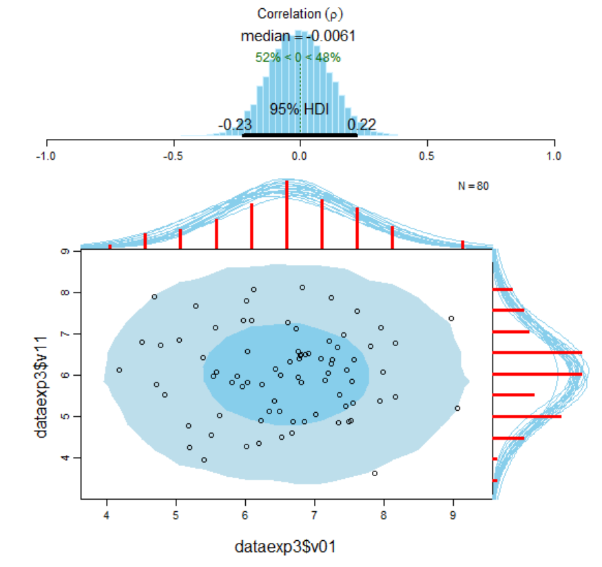
773
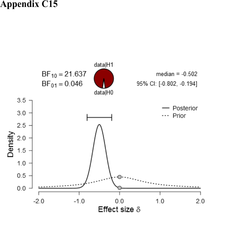
774
Inferential Plots for Bayes Factor analysis
v00 - v10
Prior and Posterior
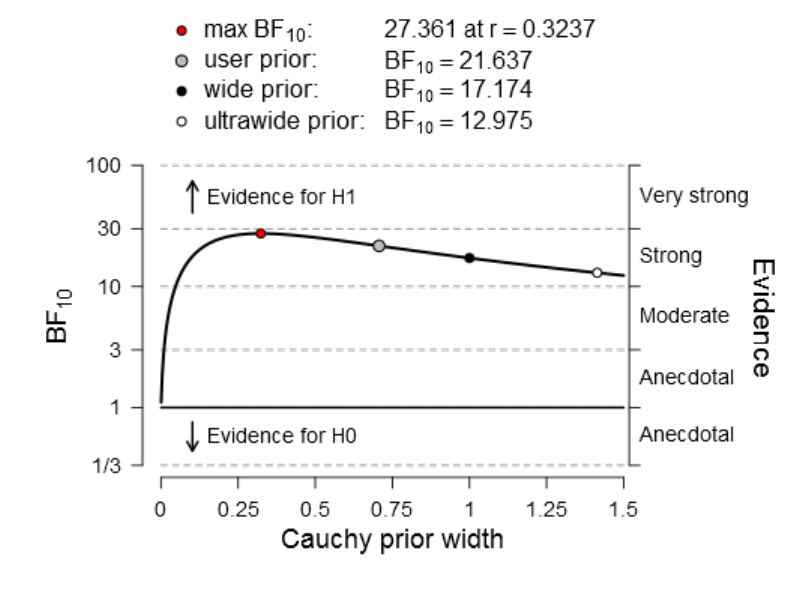
775
Bayes Factor Robustness Check
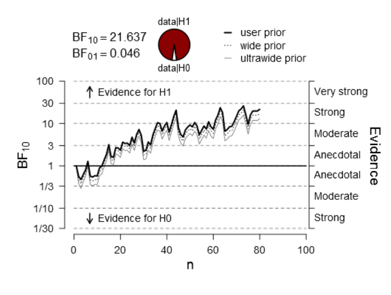
776
Sequential Analysis
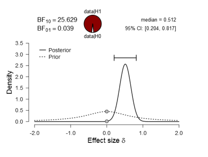
777
v01 - v11
Prior and Posterior
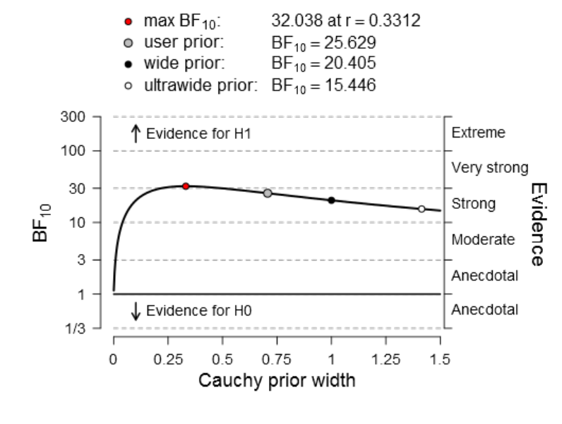
778
Bayes Factor Robustness Check
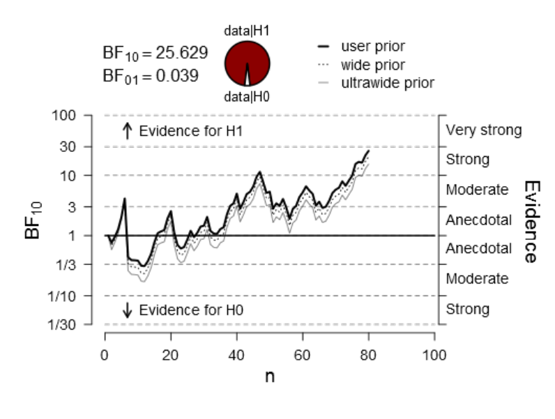
779
Sequential Analysis

780
Appendix D Experiment 3
Parametrisation of auditory stimuli
Table 58
Amplitude statistics for stimulus-0.6.wav.
Parameter
Left channel
Right channel
Peak Amplitude:
-11.54 dB
-11.60 dB
True Peak Amplitude:
-11.54 dBTP
-11.60 dBTP
Maximum Sample Value:
8674.67
8616.15
Minimum Sample Value:
-8662.86
-8612.15
Total RMS Amplitude:
-15.65 dB
-15.70 dB
Maximum RMS Amplitude:
-13.48 dB
-13.54 dB
Minimum RMS Amplitude:
-23.79 dB
-23.84 dB
Average RMS Amplitude:
-16.37 dB
-16.43 dB
DC Offset:
-0.01 %
-0.01 %
Measured Bit Depth:
24
24
Dynamic Range:
10.30 dB
10.30 dB
Dynamic Range Used:
10.20 dB
10.25 dB
Loudness (Legacy):
-13.88 dB
-13.93 dB
Perceived Loudness (Legacy):
-12.88 dB
-12.93 dB
Note. Statistics were computed by utilising Adobe© Audition CC 2017 which is part of
the Adobe Creative Suite (Adobe Systems Incorporated) and are only indicative. The
original pure tones are best replicated in PsychoPy (J. W. Peirce, 2007, 2008) using the
parametrisation “0.6” and “0.8” for the loudness parameters, respectively.

781
Table 59
Amplitude statistics for stimulus-0.8.wav.
Parameter
Left channel
Right channel
Peak Amplitude:
-0.96 dB
-1.13 dB
True Peak Amplitude:
-0.96 dBTP
-1.13 dBTP
Maximum Sample Value:
29245.00
28706.16
Minimum Sample Value:
-29334.32
-28782.39
Total RMS Amplitude:
-6.25 dB
-6.41 dB
Maximum RMS Amplitude:
-4.05 dB
-4.22 dB
Minimum RMS Amplitude:
-12.96 dB
-13.12 dB
Average RMS Amplitude:
-6.90 dB
-7.06 dB
DC Offset:
0.08 %
0.08 %
Measured Bit Depth:
24
24
Dynamic Range:
8.91 dB
8.91 dB
Dynamic Range Used:
8.85 dB
8.90 dB
Loudness (Legacy):
-4.43 dB
-4.62 dB
Perceived Loudness (Legacy):
-3.58 dB
-3.73 dB

782
Electronic supplementary materials: Auditory
stimuli
Auditory stimuli can be downloaded from the following URLs:
http://irrational-decisions.com/phd-thesis/auditory-stimuli/stimulus-0.6.wav
http://irrational-decisions.com/phd-thesis/auditory-stimuli/stimulus-0.8.wav
The original pure tones are best replicated in PsychoPy (J. W. Peirce, 2007, 2008) using
the parametrisation “0.6” and “0.8” for the loudness parameters, respectively.
PsychoPy parametrisation
sound_1 = sound.Sound('A', secs=-1)
sound_1.setVolume(0.6)
sound_2 = sound.Sound('A', secs=-1)
sound_2.setVolume(0.8)
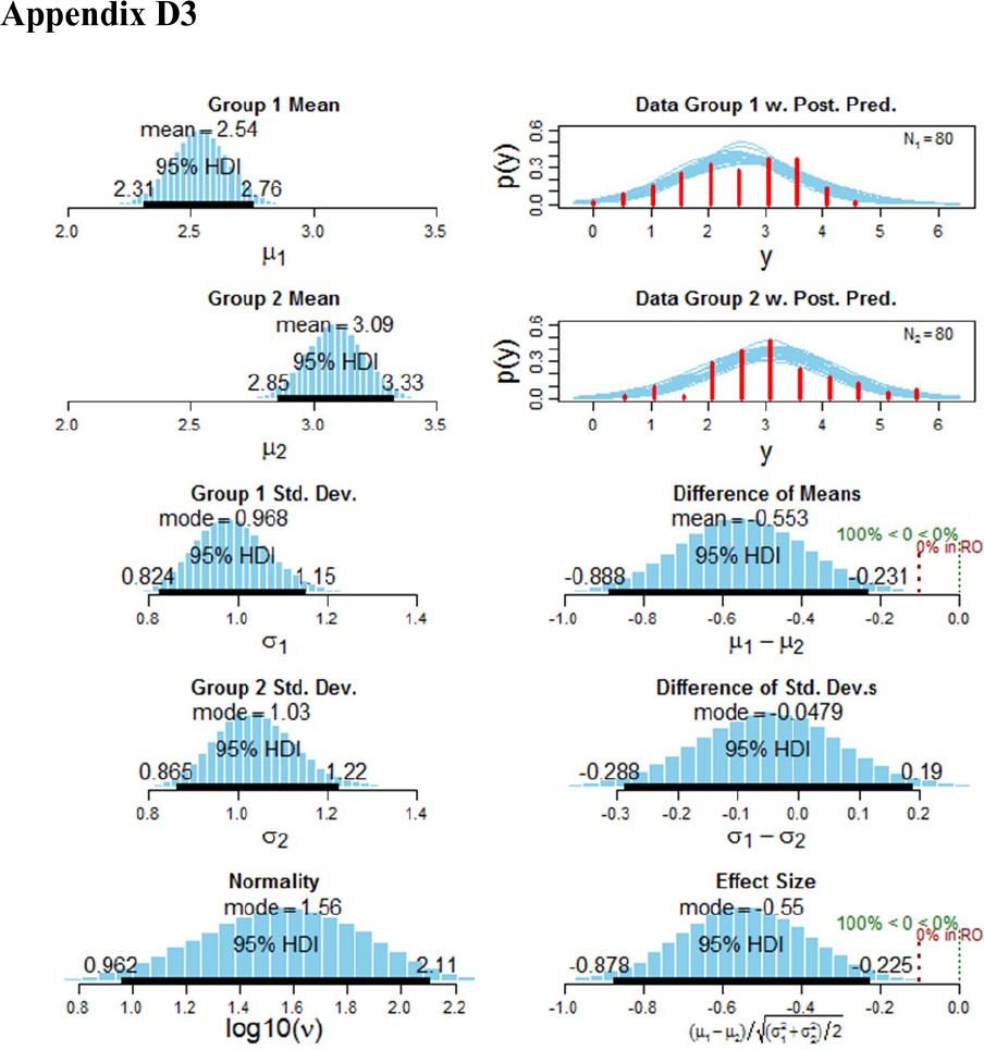
783
Bayesian parameter estimation

784
mean median mode HDI% HDIlo HDIup compVal %>compVa
l
mu1 2.5355 2.5359 2.5348 95 2.311 2.757
mu2 3.0886 3.0878 3.0870 95 2.855 3.329
muDiff -0.5531 -0.5531 -0.5579 95 -0.888 -0.231 0 0.0
4
sigma1 0.9884 0.9834 0.9680 95 0.824 1.154
sigma2 1.0392 1.0346 1.0308 95 0.865 1.225
sigmaDiff -0.0508 -0.0498 -0.0479 95 -0.288 0.190 0 33.8
6
nu 44.3790 36.0418 21.8557 95 5.149 106.906
log10nu 1.5492 1.5568 1.5611 95 0.962 2.106
effSz -0.5462 -0.5465 -0.5503 95 -0.878 -0.225 0 0.0
4
mean sd median HDIlo HDIup Rhat n.eff
mu1 2.5355 0.11433 2.5359 2.3106 2.757 1 58225
mu2 3.0886 0.12084 3.0878 2.8546 3.329 1 60056
nu 44.3790 31.21383 36.0418 5.1493 106.906 1 23284
sigma1 0.9884 0.08517 0.9834 0.8237 1.154 1 53227
sigma2 1.0392 0.09187 1.0346 0.8649 1.225 1 48718
'HDIlo' and 'HDIup' are the limits of a 95% HDI credible interval.
'Rhat' is the potential scale reduction factor (at convergence, Rhat=1
).
'n.eff' is a crude measure of effective sample size.

785
Correlational analysis
Diagnostics for first pair
Iterations = 601:33934
Thinning interval = 1
Number of chains = 3
Sample size per chain = 33334
Diagnostic measures
mean sd mcmc_se n_eff Rhat
rho -0.080 0.114 0.000 60094 1
mu[1] 2.531 0.115 0.000 59875 1
mu[2] 3.088 0.121 0.000 59789 1
sigma[1] 0.999 0.085 0.000 52540 1
sigma[2] 1.052 0.093 0.000 49827 1
nu 46.710 31.655 0.210 22849 1
xy_pred[1] 2.526 1.042 0.003 99942 1
xy_pred[2] 3.087 1.103 0.003 100343 1
mcmc_se: the estimated standard error of the MCMC approximation of the
mean.
n_eff: a crude measure of effective MCMC sample size.
Rhat: the potential scale reduction factor (at convergence, Rhat=1).
Model parameters
rho: the correlation between dataexp3$v00 and dataexp3$v10
mu[1]: the mean of dataexp3$v00
sigma[1]: the scale of dataexp3$v00 , a consistent
estimate of SD when nu is large.
mu[2]: the mean of dataexp3$v10
sigma[2]: the scale of dataexp3$v10
nu: the degrees-of-freedom for the bivariate t distribution
xy_pred[1]: the posterior predictive distribution of dataexp3$v00
xy_pred[2]: the posterior predictive distribution of dataexp3$v10
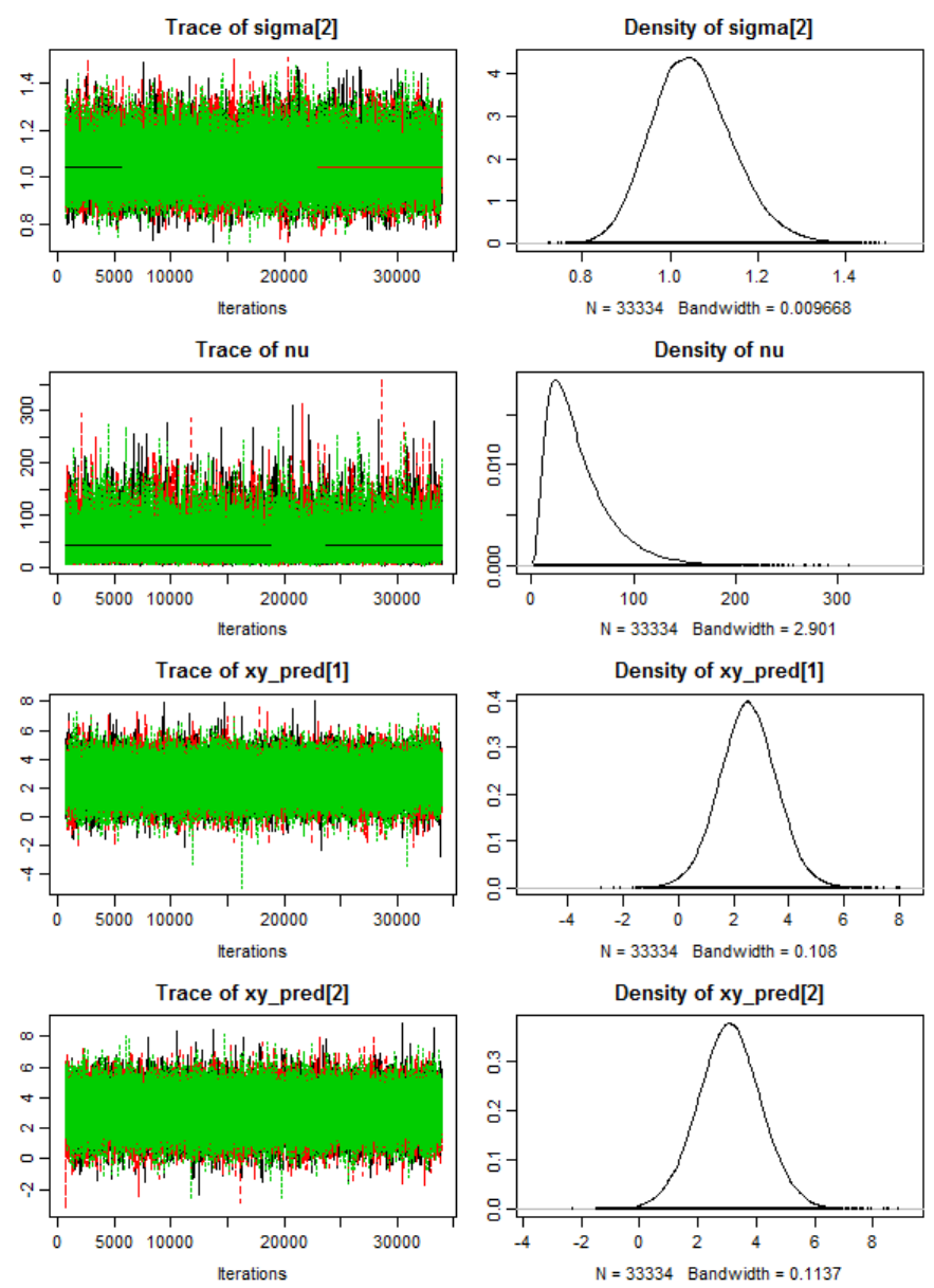
786

787
Quantiles of Bayesian correlation analysis for first pair
Quantiles
q2.5% q25% median q75% q97.5%
rho -0.299 -0.158 -0.081 -0.004 0.145
mu[1] 2.303 2.454 2.531 2.608 2.755
mu[2] 2.851 3.008 3.088 3.169 3.326
sigma[1] 0.847 0.940 0.994 1.053 1.181
sigma[2] 0.886 0.988 1.046 1.110 1.249
nu 10.172 24.065 38.521 60.742 128.927
xy_pred[1] 0.476 1.843 2.524 3.208 4.579
xy_pred[2] 0.908 2.369 3.085 3.806 5.285

788
Diagnostics for second pair
Iterations = 601:33934
Thinning interval = 1
Number of chains = 3
Sample size per chain = 33334
Diagnostic measures
mean sd mcmc_se n_eff Rhat
rho -0.006 0.115 0.000 62078 1
mu[1] 6.599 0.117 0.000 60842 1
mu[2] 6.029 0.118 0.000 61415 1
sigma[1] 1.016 0.088 0.000 49569 1
sigma[2] 1.030 0.089 0.000 52429 1
nu 46.614 31.849 0.207 23975 1
xy_pred[1] 6.601 1.068 0.003 99166 1
xy_pred[2] 6.032 1.079 0.003 100010 1
mcmc_se: the estimated standard error of the MCMC approximation of the
mean.
n_eff: a crude measure of effective MCMC sample size.
Rhat: the potential scale reduction factor (at convergence, Rhat=1).
Model parameters
rho: the correlation between dataexp3$v01 and dataexp3$v11
mu[1]: the mean of dataexp3$v01
sigma[1]: the scale of dataexp3$v01 , a consistent
estimate of SD when nu is large.
mu[2]: the mean of dataexp3$v11
sigma[2]: the scale of dataexp3$v11
nu: the degrees-of-freedom for the bivariate t distribution
xy_pred[1]: the posterior predictive distribution of dataexp3$v01
xy_pred[2]: the posterior predictive distribution of dataexp3$v11
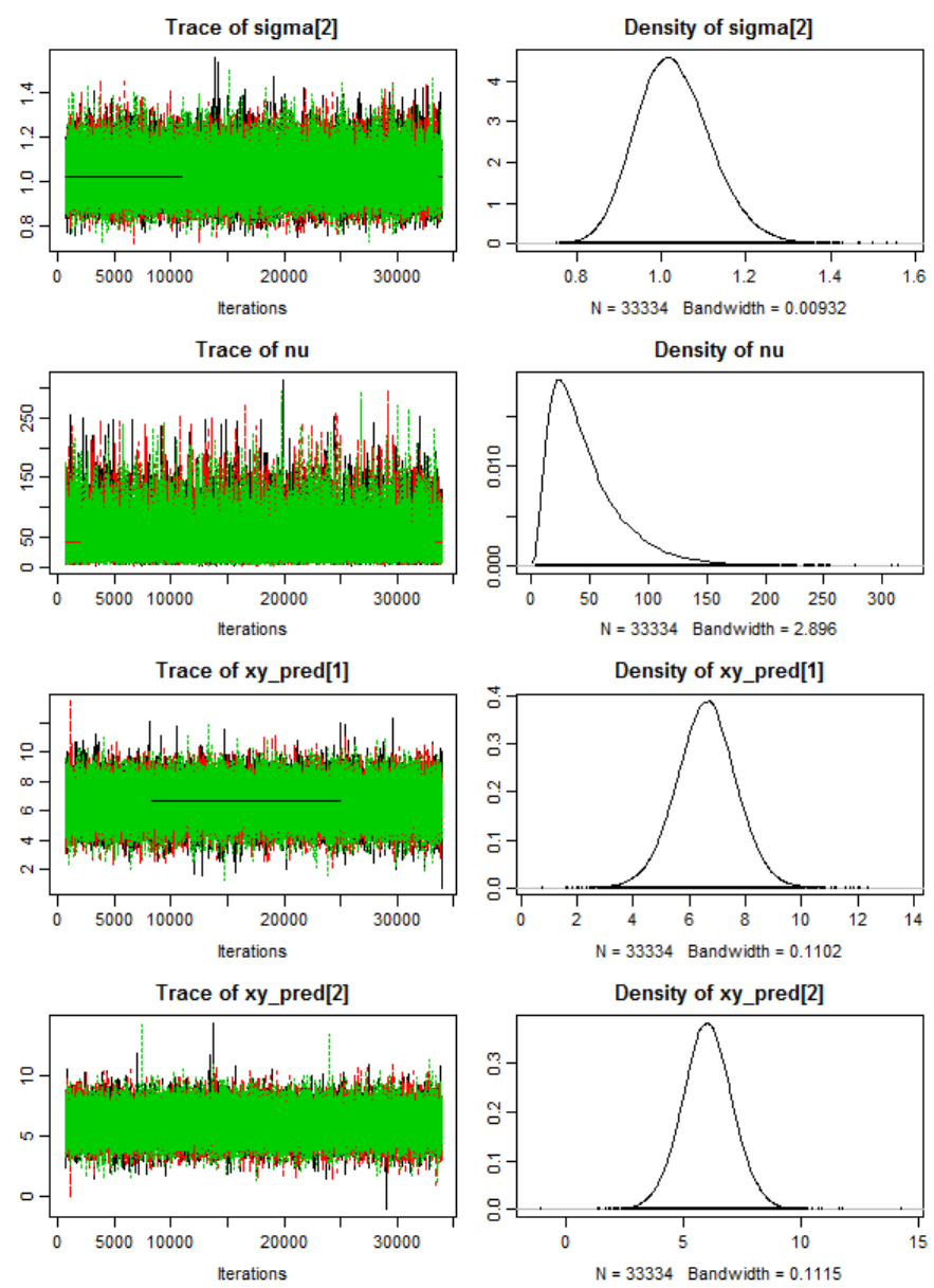
789

790
Quantiles of Bayesian correlation analysis for second pair
Quantiles
q2.5% q25% median q75% q97.5%
rho -0.231 -0.084 -0.006 0.072 0.219
mu[1] 6.370 6.521 6.599 6.678 6.827
mu[2] 5.796 5.950 6.029 6.108 6.260
sigma[1] 0.859 0.955 1.011 1.072 1.203
sigma[2] 0.871 0.969 1.025 1.086 1.218
nu 10.016 23.886 38.393 60.502 129.729
xy_pred[1] 4.471 5.908 6.607 7.301 8.691
xy_pred[2] 3.895 5.328 6.028 6.738 8.16

791
Appendix E Experiment 4
Markov chain Monte Carlo simulations
Model comparison via Bayes Factor (Bayesian confirmation theory) as described in the
antecedent chapter is thus not the only viable Bayesian alternative to classical
frequentist NHST. Bayesian parameter estimation and Bayes Factor analysis differ in
significant ways: Compared to Bayes Factor analysis, the Bayesian parameter
estimation approach provides much richer information because it results in a posterior
probability distribution on all parameters (Bayes Factor analysis does not). Model
comparison and Bayesian parameter estimation are both committed to Bayes’ theorem
as the axiomatic foundation for probabilistic inductive inferences. However, the
questions they address are fundamentally different (Steel, 2007). Whereas model
comparison is concerned with the evaluation (i.e., confirmation/rejection) of
hypotheses, Bayesian parameter estimation is primarily concerned with the computation
of posterior probability distributions for the parameters of interest. However, the
Bayesian parameter estimation approach can also be utilised to test specific research
hypotheses. In the model comparison approach, the decision (accept vs. reject) is based
on a predefined arbitrary threshold (i.e., the strength of the Bayes Factor). In the
parameter estimation approach, on the other hand, the inferential decision is based on
the specification of a threshold for the parameter under investigation (viz. a “posterior
high density interval” in combination with a “region of practical equivalence”). The
parameter estimation approach and its associated methods for hypothesis testing will be
described in more detail in the following subsections.
In sum, both Bayesian methods base the decision rule on the posterior distribution.
However, given that they focus on different facets of the posterior distribution the

792
resulting inferences do not necessarily have to coincide (Kruschke, 2014). Furthermore,
both inferential approaches are based on the notion of credence (a subjective “Bayesian”
probability describing the level of confidence or belief). Given that subjectivity involves
the epistemological idiosyncrasies and propensities of a human cogniser, credence must
be regarded as a psychological property.
In the Bayesian framework, beliefs are always provisional (as opposed to the positivist
notion of deductive absolute certainty). In the scientific sense, this means a tentative
acceptance of a theory or hypothesis combined with an explicit sense of fallibilism
245
(a
willingness to admit that the theory/hypothesis might in principle be wrong). The
explicit willingness to revise or even negate (oftentimes cherished) ideas in the light of
new evidence is a crucial aspect of genuine scientific thinking. Fallibilism is thus a
general scientific attitude towards knowledge (an epistemic virtue). The writings of the
influential philosopher of science, Karl Popper, partially agree with this epistemological
stance. His “conjecture and refutation model” of “growth of scientific knowledge”
(1962) is based on the notion that open-mindedness and intellectual humility are the
primary characteristic that render science a rational enterprise (see also C. S. Peirce,
1955).
Theoretical background of Bayesian inference
Bayesian inference has gained significantly in importance since its development in the
late 1990s, especially in the field of evolutionary biology (e.g., phylogenetic inference),
for a review see Huelsenbeck (2001). This continuing trend is visualised in Figure 129.
In general terms, Bayesian inference employs Bayes’ theorem in order to condition
245
Fallabilism asserts that a given propositions concerning empirical knowledge can be
accepted even though it cannot be conclusively proven with absolute certainty. The term is
etymologically derived from the Latin: fallibilis, meaning "liable to err" (G Gigerenzer, 1998).
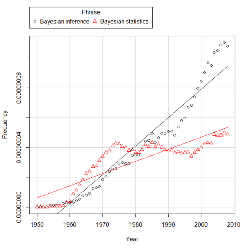
793
inferences about the numerical value of some parameter θ on the observed empirical
data (Alfaro, Zoller, & Lutzoni, 2003). The primary focus of Bayesian inference lies on
the posterior distribution or posterior probability, i.e., the probability of a given
hypothesis conditional on the empirical data.
Figure 129. Graphic depicting the frequency of the terms “Bayesian inference” and
Bayesian statistics” through time (with least square regression lines).

794
Statistics are based on various text corpora (data extracted from Google Ngram). The
visualisation was created with the R package ngramr
246
and the data visualisation
package ggplot2 (Ggplot2 Development Team, 2012; Wickham, 2009, 2011).
#ngramr manual as pdf:
#http://ftp.cs.pu.edu.tw/network/CRAN/web/packages/ngramr/ngramr.pdf
install.packages("ggplot2")
library(ggplot2)
#ggplot2 Development Team. (2012). Ggplot2-0.9.0. Production, (ii), 1–41.
#Wickham, H. (2011). ggplot2. Wiley Interdisciplinary Reviews: Computational Statistics,
3(2), 180–185. https://doi.org/10.1002/wics.147
#Wickham, H. (2009). Ggplot2. Elegant Graphics for Data Analysis.
https://doi.org/10.1007/978-0-387-98141-3
#install R developer tools
install.packages("devtools")
#get ngramr package from github repository: https://github.com/
install_github("ngramr", "seancarmody")
require(ngramr)
require(ggplot2)
require(devtools)
freq <- ngram(c("p-value", "bayes factor"), year_start = 1950)
head(freq)
summary(freq)
names(freq)
246
The manual for ngramr is available under
http://ftp.cs.pu.edu.tw/network/CRAN/web/packages/ngramr/ngramr.pdf

795
write.table(freq, "ngram_bayes.txt", sep = "\t")
ng <- ngram(c("Bayesian inference", "Bayesian statistics"), year_start = 1950)
ggplot(ng, aes(x = Year, y = Frequency, colour = Phrase)) +
geom_line() + geom_line(linetype = "dashed") +
geom_point() + theme(
panel.grid.major = element_blank(),
panel.grid.minor = element_blank(),
panel.background = element_blank(),
axis.line = element_line(colour = "black")
)
ng
#in R commander
scatterplot(
Frequency ~ Year | Phrase,
reg.line = FALSE,
smooth = FALSE,
spread = FALSE,
boxplots = FALSE,
span = 0.5,
ellipse = FALSE,
levels = c(.5, .9),
by.groups = TRUE,
data = ng
)
scatterplot(
Year ~ Frequency | Phrase,
reg.line = lm,

796
smooth = FALSE,
spread = FALSE,
boxplots = FALSE,
span = 0.5,
ellipse = TRUE,
levels = c(.5, .9),
jitter = list(x = 1, y = 1),
by.groups = TRUE,
data = ng
)
Code 10. R code to download, save, and plot data from Google Ngram. Various R
packages are required (devtools, ngramr, ggplot2).

797
While hypothesis testing plays a pivotal role in psychology and the biomedical sciences,
it is ancillary in many other scientific disciplines (e.g., physics). Many disciplines that
do not primarily rely on hypothesis testing focus on estimation and modelling. A
common problem in statistical modelling is to estimate the values of parameter of a
given probability distribution. Bayesian Parameter Estimation (BPE) methods provide a
set of powerful and robust statistical tools to obtain these values. In other words, BPE
can produce accurate approximations to the Bayesian posterior distributions of various
parameters (θ, i.e., theta) of interest. That is, parameters are modelled as probability
distributions. BPE utilises computationally expensive Markov chain Monte Carlo
(MCMC) algorithms to achieve this goal. In contrast to NHST, BPE fixes the empirical
data and instead assumes a range of credible values for θ. Moreover, BPE allows
probabilities to represent credibility (i.e., subjective certainty/belief). Hence, an
appropriate alternative nomenclature for BPE (and all other Bayesian methods) would
be “statistical uncertainty modelling”.
In the experimental context at hand, we applied Bayesian parameter estimation methods
to our empirical data in order to obtain accurate estimates of the parameter values of
interest. Based on the a priori defined hypotheses, we were particularly interested in the
posterior distribution of the means per condition, their standard deviation, and the
difference between means. BPE provides informative posterior probability distribution
for all parameters of interest.
In the subsequent subsection we will provide a brief introduction to Bayesian parameter
estimation via Markov chain Monte Carlo methods. Next, we will describe the software
packages and statistical methods we utilised for our analysis. The third section will
describe the actual Bayesian analysis and the results. This section is subdivided as
follows (according to the sequential steps of the analysis):

798
6. Definition of the descriptive model and specification of priors
7. MCMC computations of the posterior distributions
8. Diagnostics/assessment of MCMC convergence
9. Summary and interpretation of the resulting posterior distributions within the
pertinent theoretical framework
The Bayesian inferential approach we employed provides rich information about the
estimated distribution of several parameters of interest, i.e., it provides the distribution
of the estimates of μ and σ of both conditions and the associated effect sizes.
Specifically, the method provides the “relative credibility” of all possible differences
between means, standard deviations (Kruschke, 2013). Inferential conclusions about
null hypotheses can be drawn based on these credibility values. In contrast to
conventional NHST, uninformative (and frequently misleading
247
) p values are
redundant in the Bayesian framework. Moreover, the Bayesian parameter estimation
approach enables the researcher to accept null hypotheses. NHST, on the other, only
allows the researcher to reject such null hypotheses.
The critical reader might object why one would use complex Bayesian computations for
the relatively simple within-group design at hand. One might argue that a more
parsimonious analytic approach is preferable. Exactly this question has been articulated
before in a paper entitled “Bayesian computation: a statistical revolution” which was
published in the Philosophical Transactions of the Royal Society: “Thus, if your primary
question of interest can be simply expressed in a form amenable to a t test, say, there
247
For more detailed information on the frequent logically fallacious misinterpretations of p-values and
related frequentist statistics see chapter xxx.

799
really is no need to try and apply the full Bayesian machinery to so simple a problem”
(S. P. Brooks, 2003, p. 2694).
The answer is straightforward: “Decisions based on Bayesian parameter estimation are
better founded than those based on NHST, whether the decisions derived by the two
methods agree or not. The conclusion is bold but simple: Bayesian parameter
estimation supersedes the NHST t test” (Kruschke, 2013, p. 573).
Bayesian parameter estimation is more informative than NHST
248
(independent of the
complexity of the research question under investigation). Moreover, the conclusions
drawn from Bayesian parameter estimates do not necessarily converge with those based
on NHST. This has been empirically demonstrated beyond doubt by several
independent researchers (Kruschke, 2013; Rouder et al., 2009).
The juridical metaphor used before in the context of α-error inflation (see section xxx)
is also applicable in the context of Bayesian estimation. The principle of exoneration
illustrates the underlying logic of Bayesian inference. When a judge has to decide which
of two unaffiliated defendants is guilty of a crime, evidence that incriminates one
suspect automatically exonerates the other defendant. This is complementary
reallocation of probabilities according the third Aristotelian law of the excluded
middle
249
, the tertium non datur (lit. no third [possibility] is given) a.k.a. principium
tertii exclusi. The third Aristotelian “law of thought” stipulates that any given
proposition can either be true or false (there is no intermediate middle ground)
250
. It
implies that either a proposition is true, or its negation is true (Kalsi, 1994). This
248
It is also more informative than Bayes factor analysis.
249
Modern quantum physics challenges this logical postulate. We will discuss this fundamental law of
thought in chapter xxx in the context of superposition and complementarity.
250
This foundational and usually unquestioned axiom has been challenged by quantum physics (Leibfried
et al., 2005; C. Monroe, Meekhof, King, & Wineland, 1996; Schrödinger, 1935). The concepts
“superposition” and “complementarity” are discussed in chapter xxx as they play a pivotal role in the
quantum cognition paradigm.

800
principle is exemplified in a famous quote by factious consulting detective Sherlock
Holmes who is renowned for his logical reasoning and often cited by Bayesians:
“Once you eliminate the impossible, whatever remains, no matter how improbable, must
be the truth.” (Dolye, 1904)
“As in the situation of Holmesian deduction, this exoneration is not only intuitive, it is
also what the exact mathematics of Bayesian inference prescribe” (Kruschke, 2014, p.
19). For an exposition of “Bayesian thought in early modern detective stories” see
Kadane (2009). However, from an informal logic point of view this is a fallacious
argument and its form is known as the argumentam ad ignorantiam, Latin for argument
from ignorance where ignorance here means “a lack of contrary evidence,” (cf. Walton,
1992). This class of arguments fails to acknowledge one’s own epistemological
limitations (i.e., the limits of one's own understanding). In cognitive and social
psychology, being ignorant of one’s own ignorance is known as the “Dunning-Kruger
effect” (Dunning, 2011; Kruger & Dunning, 1999). Yet, in the context of Bayesian
reasoning it has been pointed out that “viewed probabilistically, these versions of the
argument from ignorance constitute a legitimate form of reasoning” (Oaksford & Hahn,
2004, p. 75). As a syllogism the argument can be represented in the following form
(modus ponens):
Major premise:
Minor premise:
Conclusion:
There is currently no evidence that p is true.
If p were true, there would be evidence.
Ergo, p is false.
This syllogism is logically valid. However, the following argument might appear
believable from a semantic point of view, but it is logically invalid:

801
Major premise:
Minor premise:
Conclusion:
There is currently no evidence that p is true.
If p were true, there would be no evidence.
Ergo, p is false.
Even though this argument might appear semantically believable, it is logically invalid.
Hence it might lead to belief-bias, an extensively studied phenomenon in the
psychology of thinking and reasoning (e.g. J. St. B. T. Evans et al., 1983). Thus, the
validity of the conclusion is conditioned on the truth or falsehood of the premises. In
Bayesian epistemology, the evidence is conditional, i.e., based on the empirical data at
hand. Carl Sagan (as cited in Stephens, 2011) gives the following example for absent
evidence reasoning: “Sherlock Holmes notices that a dog does not bark (absent
evidence) and concludes that this is evidence that there is no criminal who is stranger—
the culprit must have known the dog” (Sagan, 1997). The point Sagan wants to illustrate
that reasoning of evidence leads to fallacious logical conclusions. For instance, we
currently do not have evidence that alien intelligent life exists on other planets. Ergo,
one might conclude that there is no intelligent life on other planets. Sagan argues that
the lack of evidence does not poof the absence of alien life. On the other hand, the
absence cocaine in a standard hair follicle test is evidence that the subject under
investigation has not taken any cocaine recently.
However, a detailed discussion of “absent evidence reasoning” and the underlying
cognitive processes goes beyond the scope of this chapter and we refer the interested
reader to Stephens (2011).
From the point of view of statistical data analysis, Bayesian inference can be regarded
802
as a from of probabilistic inference that reallocates belief (credibility) across a space of
potential possibilities, i.e., a set of candidate culprits, to use the detective analogy
(Kruschke et al., 2017). The analysist (or detective or judge) is confronted with noisy
numerical data and tries to approximate the pattern with a mathematical model. “The
space of potential suspects for describing the data is the space of values for the
parameters” (Kruschke, 2013). In other words, potential suspects in legal scenario are
equivalent to a specific (plausible) range of potential parameter values in a Bayesian
descriptive model. The primary purpose of the Bayesian analysis is thus to specify a
range of possibilities (plausible parameter values) in the form of credibility intervals.

803
Mathematical foundations of Bayesian
inference
Bayesian inference allocates credibility (i.e., belief) across the parameter space Θ
251
of
the model (conditional on the a priori obtained empirical data). The mathematical
axiomatic basis is provided by Bayes’ theorem. Bayes’ theorem derives the probability
of θ given the empirical data in terms of its inverse probability (i.e., the probability of
the data given θ and the prior probabilities of θ). In other word “Bayesian data analysis
involves describing data by meaningful mathematical models, and allocating credibility
to parameter values that are consistent with the data and with prior knowledge”
(Kruschke & Vanpaemel, 2015, p. 279)
The mathematical formula for the allocation of credibility across parameters is
axiomatized in Bayes’ theorem (Bayes & Price, 1763), i.e., Bayes’ theorem
mathematically defines the posterior distribution on the parameter values in a formal
manner.
(|) =
(|) ()
()
Where:
• () signifies the prior (the preliminary belief about A)
• () signifies the evidence
• (|) signifies the posterior probability (the belief about of A given B)
• (|) signifies the likelihood.
251
Uppercase Theta (Θ) denotes the set of all possible combinations of parameter values in a specific
mathematical model (the joint parameter space). Lowercase theta (θ) on the other hand, denotes a single
k-dimensional parameter vector.

804
Applied to the current analysis Bayes’ theorem takes the following form:
(
,
,
,
,
|
)
= ( |
,
,
,
, )
x (
,
,
,
, )
/ ()
let D be the empirical data, μ
1
and μ
2
the means per experimental condition (e.g.,
condition V
00
and V
01
), σ
1
and σ
2
the associated standard deviations, and the
normality parameter.
Bayes’ theorem (Bayes & Price, 1763) as specified for the descriptive model used to
estimate the parameters of interest in Experiment 2.
Bayes’ theorem emphasises the posterior (conditional) distribution of parameter values
(the Latin terminus “a posteriori” signifies empirical knowledge which proceeds from
experiences/observations). The factors of Bayes’ theorem have specific meaning
assigned to them: The “evidence” for the specified model, p(D), equals the total
probability of the data under the model which can be computed by averaging over the
parameter space Θ (Kruschke, 2015). Each parameter value is weighted by the “strength
of belief” in the respective values of θ. For the current model, Bayes’ theorem can be
semantically summarised as follows: It signifies that the posterior probability of the
combination of parameter values (i.e., < μ
1
, μ
2
, σ
1
, σ
2
, >) is equal to the likelihood of
that parameter value combination multiplied by the prior probability of that parameter
combination, divided by the constant p(D). This constant is often referred to as the
“evidence” for the model and is also called the “marginal likelihood function”
(Kruschke, 2013). Its numerical value is calculated by taking the average of the
likelihood, p(D|θ), across all values of θ (i.e., over the entire parameter space Θ),
weighted by the prior probability of θ (Kruschke, 2014). The posterior distribution is

805
thus always a compromise between the prior believability of the parameter values and
the likelihood of the parameter values, given data. (Kruschke, 2010b). Our experimental
data was measured on a visual analogue scale (VAS) ranging across a continuum of
values. Given the extremely fine-grained nature of our measurements the resulting
numerical values are “quasi-continuous”. Therefore, all parameters are regarded as
continuous variables for all practical purposes. It thus follows that the posterior
distribution is continuously distributed across the joint parameter space Θ (Kruschke et
al., 2017).
Given that Bayesian parameter estimation (BPE) is currently no methodological
standard in psychology we will provide some terminological clarifications of the
underlying Bayesian nomenclature. The credibility of the parameter values after the
empirical observation is termed the “posterior distribution”, and the believability of the
parameter values before the empirical observation is termed the “prior distribution”. The
probability of the observation for a particular parameter value combination, is called the
“marginal likelihood function”. It indicates the degree to which the observed outcome is
anticipated, when averaged across all possible values of the weights, scaled
proportionally to their respective believability (Kruschke, 2008). The denominator
labelled as “evidence”, p(D), is the marginal likelihood also referred to as “model
evidence”. In BPE, Bayes’ theorem is used to make inferences about distribution
parameters, i.e., the conditional distribution of θ is calculated given the observed data.
What is the probability of θ conditional on the observed data. The prior is an
unconditional distribution associated with θ. In contrast to NHST, θ is not assumed to
be random, we are merely nescient
252
of its value. In other words, probability is
252
The term “nescienct” is a composite lexeme composed of the Latin prefix from ne "not" + scire "to
know" (cf. “science”). It is not synonymous with ignorant because ignorance has a different semantic
meaning (“to ignore” is very different from “not knowing”).
806
conceptualised as a state of subjective belief or state of knowledge (as opposed to
objective “pure” probability as an intrinsic characteristic of θ).
The posterior distribution is approximated by a powerful class of algorithms known as
Markov chain Monte Carlo (MCMC) methods (named in analogy to the randomness of
events observed at games in casinos). MCMC generates a large representative sample
from the data which, in principle, allows to approximate the posterior distribution to an
arbitrarily high degree of accuracy (as ). The MCMC sample (or chain) contains a
large number (i.e., > 1000) of combinations of the parameter values of interest. Our
model of perceptual judgments contains the following parameters: < μ
1
, μ
2
, σ
1
, σ
2
, >.
In other words, the MCMC algorithm randomly samples a very large n of combinations
of θ from the posterior distribution. This representative sample of θ values is
subsequently utilised in order to estimate various characteristics of the posterior
(Gustafsson et al., 2017), e.g., its mean, mode, standard deviation, etc. pp. The thus
obtained sample of parameter values can then be plotted in the form of a histogram in
order to visualise the distributional properties and a prespecified high density interval
can be superimposed on the histogram.
Relatively recent advances in technology make these computationally demanding
methods feasible. The combination of powerful microprocessor and sophisticated
computational algorithms allows researchers to perform extremely powerful Bayesian
statistical analyses that would have been very expensive only 15 years ago and virtually
impossible circa 25 years ago. The statistical “Bayesian revolution” is relevant for many
scientific disciplines (Beaumont & Rannala, 2004; S. P. Brooks, 2003; Gregory, 2001;
Shultz, 2007) and the scientific method in general. This Kuhnian-paradigm shift (T.
Kuhn, 1970) goes hand in hand with the Moore's law (G. E. Moore, 1965) and the
exponential progress of information technologies (Kurzweil, 2005) (cf. Goertzel, 2007)

807
and the associated ephemeralization
253
(Heylighen, 2008). This topic is discussed in
greater detail in chapter xxx.
For the current Bayesian analysis, the parameter space Θ is a five-dimensional space
that embeds the joint distribution of all possible combinations of parameter values
(Kruschke, 2014). Hence exact parameter values can be approximated by sampling
large numbers of values from the posterior distribution. The larger the number of
random samples the more accurate the estimate. A longer MCMC chain (a larger
sample) provides a more accurate representation (i.e., better estimate or higher
resolution) of the posterior distribution of the parameter values (given the empirical
data). For instance, if the number of MCMC samples is relatively small and the analysis
would be repeated the values would be significantly different and, on visual inspection,
the associated histogram would appear “edgy”. With larger MCMC samples, the
estimated values (on average) approximate the true values of the posterior distribution
of the parameter values and the associated histogram becomes smoother (Kruschke,
2014). The larger the MCMC sample size the higher the accuracy because the sample
size n is proportional to the “Monte Carlo Error” (MCE; i.e., accuracy is a function of
MCMC sample size). To sum up, the MCMC approach clearly yields approximate
parameter values and its accuracy depends on the number of values n that are used to
calculate the average. Quantitative methods have been developed to measure the Monte
Carlo Error “objectively” (Elizabeth Koehler, Elizabeth Brown, 2009), however, this
intricate topic goes beyond the scope of this chapter. Of great relevance for our purpose
is the fact that this analytic approach also allows to compute the credible difference of
means between experimental conditions by computing μ
1
- μ
2
for every combination of
253
A concept popularised by Buckminster Fuller which is frequently cited as an argument against
Malthusianism.

808
sampled values. Moreover, BPE provides a distribution of credible effect sizes. The
same distributional information can be obtained for the differences between σ
1
and σ
2
(and the associated distributional range of credible effect sizes). To sum up, BPE is
currently one of the most effective statistical approaches to obtain detailed information
about the various parameters of interest.
Markov chain Monte Carlo (MCMC)
methods
Markov Chain Monte Carlo have transformed science, particularly due to their
relevance for probabilistic logical inferences. Monte Carlo methods (sometimes termed
Monte Carlo experiments) are a class of computational algorithms that utilise repeated
random sampling to calculate their statistical results. The theoretical considerations
behind Monte Carlo methods are old, for an example see the Buffon-Laplace need
problem (Buffon, 1777). The appellation “Monte Carlo” is frequently attributed to the
quantum physicist John von Neumann (inter alia) and Monte Carlo methods have been
discussed in many diverse scientific contexts (Behrends, 2014; Dell & Franklin, 2009;
Diaconis, 1976). However, they are generally primarily applied to three broad classes of
problems: mathematical optimization, numerical integration, and the generation of
samples from probability distributions (Kroese, Brereton, Taimre, & Botev, 2014).
Markov chains are based on the stochastic foundations developed by the Russian
mathematician Andreyevich Markov who extended the central limit theorem to
sequences of random variables (hence the eponymous name “Markov chains”). In 1912,
his work was translated into German under the title “Wahrscheinlichkeitsrechnung“,
that is “probability calculus” (Markov, 1912). For a historical overview see Basharin,
Langville, & Naumov (2004).
Markov chain Monte Carlo methods are based on the seminal work of the physicist

809
Nicholas Metropolis et alia (Metropolis, Rosenbluth, Rosenbluth, & Teller, 1953) who
initially utilised the approach to simulated energy levels of atoms in crystalline
structures
254
. The concept was later generalised by the statistician W. K. Hastings
(1970). MCMC methods became more popular in the context of Bayesian inference due
to the work of Gelfand and Smith (1990) who emphasised the relevance of MCMC
methods to calculating Bayesian posterior densities. Recent computational advances
have made them more accessible to researchers in various scientific disciplines
(Diaconis, 2008; W. L. Dunn & Shultis, 2012). Today, the Metropolis–Hastings
algorithm is one of the most widely used MCMC algorithm in statistics and in statistical
physics. The Metropolis–Hastings algorithm comprises the construction of a Markov
process which, in theory, results in a unique and stationary distribution. For a detailed
mathematical derivation of the algorithm see Robert and Casella (2004). Gibbs
sampling can be regarded as a special case of the Metropolis–Hastings algorithm .
Hence, MCMC methods based on the Gibbs sampling enables the analyst to draw
inferences from iterative simulations (Gelman & Rubin, 1992). The quality of MCMC
sample improves as a function of the number of steps. MCMC methods thus provide
sampling probability density functions which can be utilised to obtain parameter
estimates with their probabilistic associated uncertainties. To be specific, the goal of the
MCMC method is to obtain a large set of samples (θ
l
, l = 1, …, L) from the posterior
distribution in order to be in a position to estimate the parameters in question with
254
Currently, cutting-edge Monte Carlo-based methods are applied to simulate complex quantum
systems. The application of Monte Carlo methods to quantum physics is termed “Quantum Monte Carlo”
(QMC). QCM has been used to approximate the statistical properties of bosons and fermions and it comes
in various flavours. However, its foundation is based on the original seminal publication by Metropolis et
al. (1953) titled “Equation of State Calculations by Fast Computing Machines” in which the authors
suggested that Monte Carlo methods could in principle be utilised for “calculating the properties of any
substance” (p.1087). Simulated Quantum Annealing (SQA) is a Markov Chain Monte-Carlo algorithm
that has been utilised to simulating quantum annealing. In addition, SQA can be applied to
multidimensional combinatorial optimization problems and it has been argued that it inherits some of the
advantages of quantum tunnelling (but see Crosson & Harrow, 2016).
810
reasonable accuracy. As a general heuristic rule, it has been stated that L =100 is
sufficient for reasonable posterior estimates. (Gelman et al., 2004). A sample that is too
small can lead to inaccurate statistical inference. Stopping rules have been developed
(Gong & Flegal, 2016) and the size of the Monte Carlo sample effects the standard
error. Several convergence diagnostics have been developed. The Monte Carlo Error
(MCE) is the uncertainty which can be attributed to the fact that the number of
simulation draws is always finite. In other words, it provides a quantitative index that
represents the quality of parameter estimates. For more information on the Markov
chain central limit theorem see Jones (2004). The MCSE package in R provides
convenient tools for computing Monte Carlo standard errors and the effective sample
size (James Flegal et al., 2017). Notice that relatively small MCSEs indicate high
estimation precision level. The main idea is to terminate the simulation when an
estimate is sufficiently accurate for the scientific purpose of the analysis. Many
practitioners utilize convergence diagnostics and visual inspections to evaluate if the
chain has been run long enough.
In sum, MCMC are utilised to estimate characteristics of a posterior distribution by
constructing a Markov chain with the target as its equilibrium distribution.

811
Software for Bayesian parameter estimation
via MCMC methods
In order to conduct the Bayesian parameter estimation, we utilised several open-source
software packages (all are all freely available on the internet). We created a website
were the associated URLs are compiled: http://irrational-decisions.com/?page_id=1993
Analyses were entirely conducted in R using the “BEST” package (Kruschke, 2014).
Best is an acronym for “Bayesian Estimation Supersedes the t-Test”. Moreover, we
installed JAGS “Just Another Gibbs Sampler” (Plummer, 2003, 2005) and RStudio
(RStudio Team, 2016). BEST has numerous (recursive) reverse dependencies and
reverse import dependencies which can be found with the code below. For example, it
relies on the software BUGS
255
“Bayesian inference Using Gibbs Sampling” (Lunn,
Spiegelhalter, Thomas, & Best, 2009; Spiegelhalter, Thomas, Best, & Lunn, 2014). The
utilised programs have been described in great detail two recent textbooks on Bayesian
analysis (Kruschke, 2010a, 2014).
255
The BUGS project is hosted by the MRC Biostatistics Unit, University of Cambridge:
https://www.mrc-bsu.cam.ac.uk/software/bugs/

812
R code to find various dependencies of the
“BEST” package.
install.packages("miniCRAN")
library("miniCRAN")
tags <- "BEST"
pkgDep(tags, suggests = TRUE, enhances = TRUE)
Code 11. R code to find various dependencies of the “BEST” package.

813
Hierarchical Bayesian model
In order to carry out the Bayesian parameter estimation procedure, we first defined the
prior distribution. The to be estimated parameters relevant for the hypotheses at hand
were: the means μ
1
and μ
2
; the standard deviation σ
1
and σ
2
and the normality parameter
ν. We were particularly interested in the a priori predicted difference between
experimental conditions, i.e., μ
1
– μ
2
. The main purpose of the Bayesian parameter
estimation was thus to estimate these parameters and to quantify the associated
uncertainty (i.e., credibility) of these approximations. We defined a descriptive model
for the Bayesian parameter estimation which is outlined in the following subsection. We
ascribed an appropriate prior distribution to all five parameters (see Figure 130). The
prior distribution specified for each parameter is as follows: The empirical data () is
described by a t-distribution (the wider tails make the t-distribution more robust
compared to the Gaussian distribution, i.e., it is less sensitive to outliers). The t-
distribution has three parameters: the mean (μ), the scale parameter (σ), and the degrees
of freedom (ν). Low values of ν are associated with wider tails (ν can be regarded as a
“shape parameter”). As ν get larger the t-distribution converges to a Gaussian (see
Figure 131 and Figure 132).
In order to make the prior distribution tolerable for a sceptical audience we chose very
unspecific priors which signify a lack of prior knowledge about the conceivable values
of the parameters of interest. Defining the prior distribution in such vague
(noncommittal) terms indicates that it has a negligible impact on the estimation of the
posterior distribution. In other words, by choosing noninformative priors we ensured
that the data governs the inference.
All priors were specified according to the model detailed in Kruschke (2013). The prior

814
distribution of μ
1
and μ
2
was defined as a very broad normal distribution in the model.
The standard deviation S of the prior distribution of μ
1
and μ
2
was arbitrarily defined as
1000 times the standard deviation of both conditions (i.e., SD
pooled
). Moreover, the mean
M of the prior distribution was defined in the same way (1000*pooled
{,
}). The prior of the standard deviation parameters σ
1
and σ
2
was likewise
defined with noncommittal characteristics, ranging from a low value L (one thousands
of the standard deviation of the pooled conditions) to a high value H. We ascribed an
exponentially distributed prior to parameter. This configuration distributes prior
credibility relatively homogenously over Gaussian and heavy-tailed data distributions.
In doing so we followed the recommendation described in (Kruschke, 2013, Appendices
A and B). For precise mathematical derivations see Krusckke (2014).
Definition of the descriptive model and
specification of priors
The parameters μ1 and μ2 are modelled by a normal distribution. In concordance with
Kruscke (2013) the standard deviation of μ was expressed in very broad terms
(SDpooled x 1000). The mean M of the prior distribution of μ was defined a M
pooled
(the
pooled mean of the empirical data). The prior distribution for σ
1
and σ
2
was also
noninformative, i.e., a wide uniform distribution with hyperparameters ranging from
L=SDpooled /1000 to H 1000xSD
pooled
. In practical terms, the resulting priors are
extremely wide and approximate a uniform distribution raging from -∞ to ∞. Lastly, the
prior distribution for a shifted exponential (λ=29, shifted+1) was defined for the
normality index ν (for mathematical details see Kruschke, 2013, Appendix A). As a
simplifying assumption, it is postulated that the degree of normality ν is equivalent for
both experimental conditions. The probabilistic model is visualised in Figure 130.
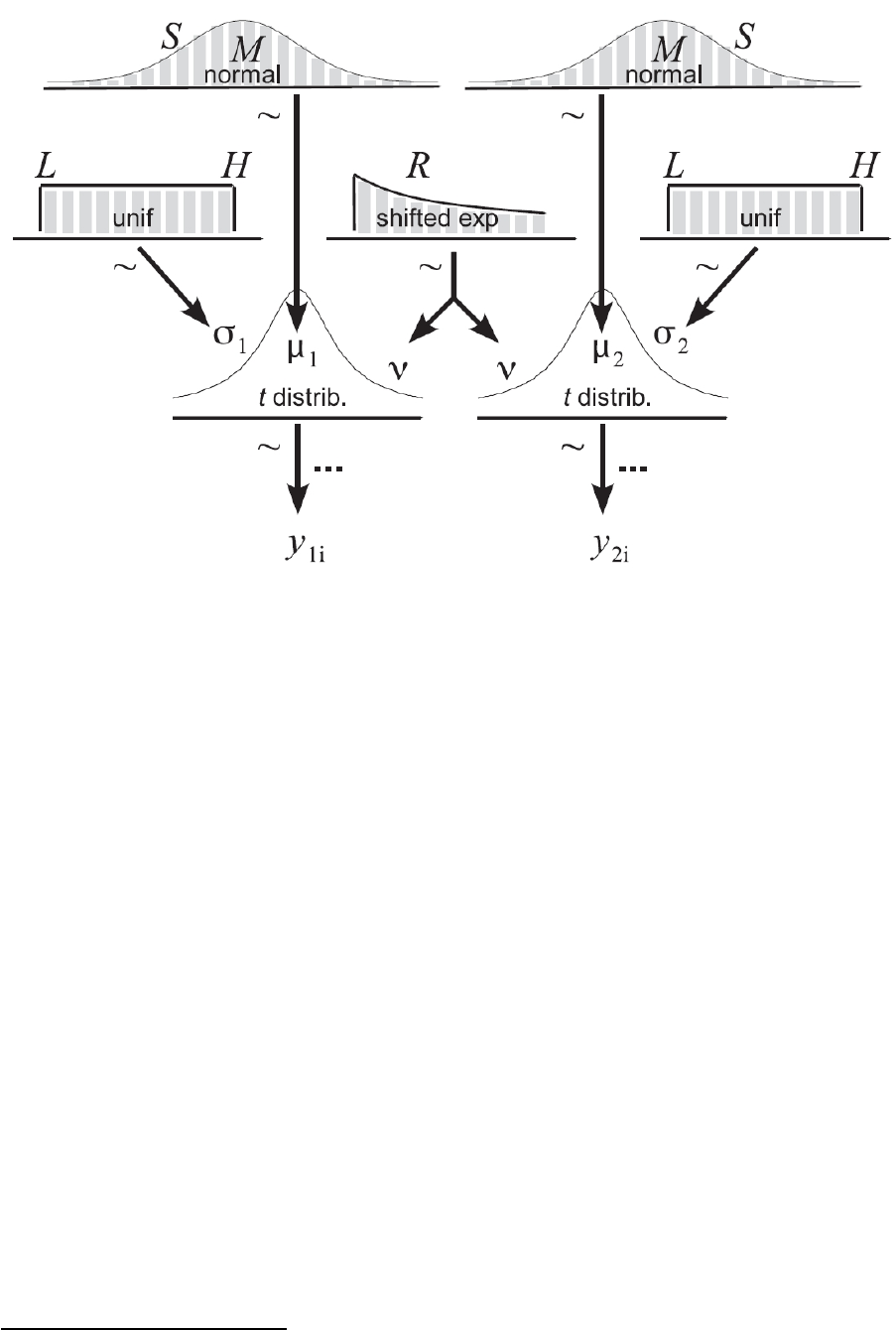
815
Figure 130. Hierarchically organised pictogram of the descriptive model for the
Bayesian parameter estimation (adaptd from Kruschke, 2013, p. 575).
The experimental data from condition V
00
(yli) and V
01
(y2i) are located at the bottom
of the pictogram. These data are described by heavy tailed and broad (noncommittal) t-
distributions
256
. The data are randomly distributed (~) and the conditions have unique
parameters for the respective means and standard deviations, i.e., μ
1
, μ
2
, and σ
1
, σ
2
,
correspondingly. The parameter for the normality index v is equivalent and thus shared
between conditions. Summa summarum, we defined four unique types of distributions
for the five-dimensional parameter space Θ. The respective distributions were
parametrised in such a way that prior commitment has a minimal impact on the
posterior (i.e., we adopted a non-informative “objective” Bayesian approach).
256
Note that the t-distribution is stipulated as the distribution for the data. By contrast, the NHST t-test
utilises the t-distribution as a distribution of the sample mean divided by the sample standard deviation.
816
Legend:
• S = standard deviation;
• M = mean;
• L =low value;
• H = high value;
• R = rate;
• unif = uniform;
• Shifted exp = shifted exponential;
• distrib. = distribution

817
Figure 131. Visual comparison of the Gaussian versus Student distribution.

818
curve(dnorm(x), -10, 10, n=1000, col = "red", ylab="")
curve(dt(x, df = 3), col = "blue", add = TRUE)
legend("topright", c("Gaussian","T"),
lty=c(1,1,1), # symbols (lines)
lwd=c(2,2,2), col=c("red", "blue"))
Code 12. R code for visualising a Gaussian versus Student distribution.
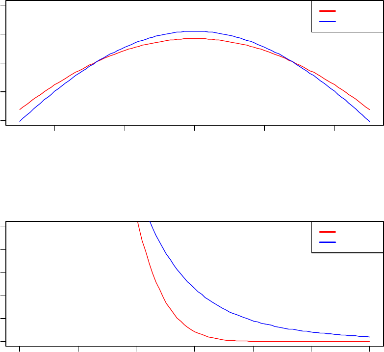
819
Figure 132. Visual comparison of the distributional characteristics of the Gaussian
versus Student distribution.
-0.4 -0.2 0.0
0.2 0.4
0.90 0.95 1.00 1.05 1.10
x
Gaussian
T
0 1 2 3 4 5 6
0.00 0.02 0.04
x
Gaussian
T

820
layout(matrix(c(1,1,2,2), 2, 2, byrow = TRUE))
df <- 3
a <- 0.5
cond_norm_dist <- function(x) dnorm(x)/(pnorm(a) - pnorm(-a))
cond_t_dist <- function(x) dt(x, df = df)/(pt(a, df = df) - pt(-a,
df = df))
curve(cond_norm_dist(x), -a, a, col = "red", ylab="")
curve(cond_t_dist(x), col = "blue", add = TRUE)
legend("topright", c("Gaussian","T"),
lty=c(1,1,1), # symbols (lines)
lwd=c(2,2,2), col=c("red", "blue"))
#zoom in on tail to emphasise heavy tail of t distribution
low <- 0; high <- 6
curve(dnorm(x), from = low, to = high, ylim = c(0, .05), col = "red", ylab="")
curve(dt(x, df = 3), col = "blue", add = TRUE)
legend("topright", c("Gaussian","T"),
lty=c(1,1,1), # symbols (lines)
lwd=c(2,2,2), col=c("red", "blue"))
Code 13. R code for detailed comparison of differences between the Gaussian and the
superimposed t-distribution.
As can be seen in Figure 131 and Figure 132 the Student t-distribution (invented by
Gosset, 1908; a.k.a. Student)
257
is more centred around 0. In comparison to the Gaussian
distribution, the t-distribution has heavy tails. The height of the tails is denoted by the
Greek letter ν (nu). A heavy-tailed distribution has a large (e.g., a value of 90). A
small on the other hand, signifies an approximation of the Gaussian distribution.
257
For a historical discussion see Fisher-Box (1987; 1981) and Neyman (1938).
821
Hence, can be regarded as a quantitative tail-index of a given probability density
function. If has a small parameter, the distribution can represent data with outliers
very well. In the subsequent analysis, data from each experimental condition will be
described with a t distribution. Each condition has its individual mean and standard
deviation. Because we did not observe many extreme values (i.e., spurious outliers) we
will use an identical tail-index ν for both conditions. In sum, we will utilise Bayesian
estimation for the following five parameters: μ
1
, μ
2
, σ
1
, σ
2
, and .

822
Summary of the model for Bayesian
parameter estimation
The specified model describes the data with five parameters: < μ
1
, μ
2
, σ
1
, σ
2
, >. The
priors were very vaguely defined. Noncommittal priors have the advantage that the
parameter estimates are primarily determined by the empirical data (i.e., bottom-up/data
driven inference) and not by a priori theoretical considerations which might bias the
model. The analysis will produce thus produce five parameter estimates that are
statistically plausible given the experimental data at hand.
We parametrised the model with default (noninformative priors), specifically we
defined normal priors with a large minimally informative standard deviation for μ,
uniform minimally informative priors for σ, and an minimally informative exponential
prior for v. Mathematical details about this specification are provided in chapter 11 and
12 in (Kruschke, 2015).
823

824
MCMC computations of the posterior
distributions
Bayesian posterior probabilities were calculated via Markov chain Monte Carlo
sampling in order to compare differences between experimental conditions. We
executed the program in the following way:
1. We loaded the function “BEST.R” into R's working memory (the function has
several dependencies and several programmes need to be installed in advance,
e.g., it relies on JAGS and BUGS and RStudio should be installed).
2. The experimental data was downloaded from the specified URL and formatted
into the first two condition (V00 and V01) were converted into vectors.
3. A MCMC chain of the length of 100,000 was generated
4. The results were plotted
5. The numerical output was generated
The associated R code can be downloaded from the following URL: http://irrational-
decisions.com/?page_id=1996

825
Reproducible analysis scrips for the simulations and analyses are available under the
following URL: http://irrational-decisions.com/phd-thesis/
##########################################################################
######
### To run this program, please prepare your computer as follows.
### 1. Install the general-purpose programming language R from
### http://www.r-project.org/
### Install the version of R appropriate for your computer's operating
### system (Windows, MacOS, or Linux).
### 2. Install the Bayesian MCMC sampling program JAGS from
### http://mcmc-jags.sourceforge.net/
### Again, install the version appropriate for your operating system.
### 3. Install the R editor, RStudio, from
### http://rstudio.org/
### This editor is not necessary, but highly recommended.
### 4. Make sure that the following programs are all
### in the same folder as this file:
### BESTexample.R (this file)
### BEST.R
### DBDA2E-utilities.R
### BESTexamplePower.R
### 5. Make sure that R's working directory is the folder in which those
### files reside. In RStudio, use menu tabs Tools -> Set Working Directory.
### If working in R, use menu tabs File -> Change Dir.
### 6. After the above actions are accomplished, this program should
### run as-is in R. You may "source" it to run the whole thing at once,
### or, preferably, run lines one at a time in order.
##########################################################################
######

826
#clears all of R's memory
rm(list=ls())
# Get the functions loaded into R's working memory
# The function can also be downloaded from the following URL:
# http://irrational-decisions.com/?page_id=1996
source("BEST.R")
#download data from server
dataexp2 <-
read.table("http://www.irrational-decisions.com/phd-thesis/dataexp2.txt",
header=TRUE, sep="", na.strings="NA", dec=".", strip.white=TRUE)
# Specify data as vectors
y1 = c(dataexp2$v00)
y2 = c(dataexp2$v01)
# Run the Bayesian analysis using the default broad priors described by Kruschke (2013)
mcmcChain = BESTmcmc( y1 , y2 , priorOnly=FALSE ,
numSavedSteps=12000 , thinSteps=1 , showMCMC=TRUE )
postInfo = BESTplot( y1 , y2 , mcmcChain , ROPEeff=c(-0.1,0.1) )
Code 14. R code for Bayesian analysis using the “BEST.R” function.

827
The function “BEST.R” can be downloaded from the CRAN (Comprehensive R
Archive Network) repository under https://cran.r-
project.org/web/packages/BEST/index.html or from our website under the following
URL: http://irrational-decisions.com/?page_id=1996
Alternatively, the BEST function has been ported to MATLAB
258
and Python.
259
The BEST core function (BESTmcmc) was implemented to obtain the Monte Carlo
based estimations of all posterior quantities of interest. In order to achieve a robust
(stable) MCMC approximation of the posterior, we specified a Markov chain length of
100,000. We saved a total length of 12,000 after adaption of 500 steps and burn-in of
1000 steps. Moreover, we thinned the chain by 5 to counteract autocorrelation. This
procedure resulted in a data matrix of 1200 rows and 5 columns, i.e., one column for
each of the five parameters of interest < μ
1
, μ
2
, σ
1
, σ
2
, >. In order to ensure that the
MCMC approach yields and accurate representation of the posterior distribution we
conducted several diagnostic tests of convergence which are reported in the following
subsection.
258
Matlab version of BEST: https://github.com/NilsWinter/matlab-bayesian-estimation/
259
Python version of BEST: https://github.com/strawlab/best/

828
MCMC convergence diagnostics
To visualise the dataset which resulted from the MCMC sampling we created a 3D-
scatterplot. The resulting graphics are depicted in Figure 122. The depiction of the
entire parameter space Θ would require a 5-dimensional representation which is
obviously impossible to visualise.
Gibbs sampling is a Markov chain Monte Carlo algorithm for obtaining a sequence of
random samples (based on a random walk model) from a priori defined probability
distribution. Specifically, Gibbs sampling is a special case of the Metropolis-Hastings
algorithm (Hastings, 1970). Gibbs sampling is a widely used methods in the context of
Bayesian inferential statistics.
As discussed previously in the context of quantum probability and superposition
(Chapter xxx), a (first-order) Markov process is a memoryless random walk (no
memory of the previous state), i.e., its past and future states are stochastically
independent (Gagniuc, 2017). A sequential succession of such steps is a Markov chain
(eponymously named after Andrey Markov).
The MCMC method used in the subsequent analysis to automatically fine-tune the
Markov chain parameters is based on an adaptive Metropolis-within-Gibbs algorithm. A
detailed description of the mathematical underpinnings of this method is given by (G.
O. Roberts & Rosenthal, 2009). Theoretically (based on the law of large numbers), as
time approximates infinity (t ) a given Markov chain will converge to a stationary
distribution (after the prespecified burn-in period (Geman & Geman, 1984)). This
stationary distribution is also called the equilibrium distribution. In Bayesian inferential
statistics, the equilibrium distribution forms the posterior distribution.
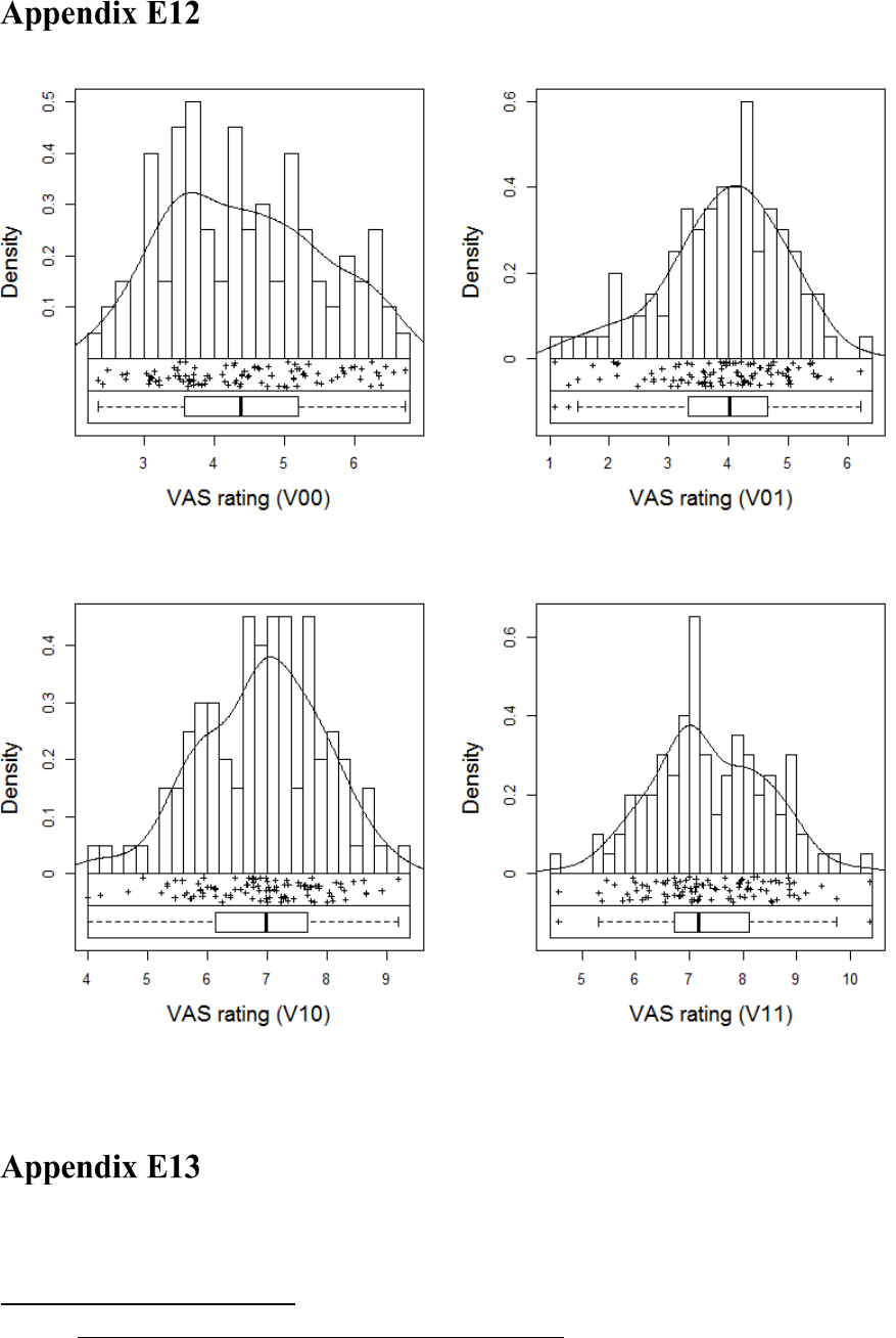

830
After (Filliben, 1975)
data: dataexp4$v00
ppcc = 0.98922, n = 100, p-value = 0.0938
alternative hypothesis: dataexp4$v00 differs from a Normal distribution
data: dataexp4$v01
ppcc = 0.98878, n = 100, p-value = 0.0857
alternative hypothesis: dataexp4$v01 differs from a Normal distribution
data: dataexp4$v10
ppcc = 0.99521, n = 100, p-value = 0.6184
alternative hypothesis: dataexp4$v10 differs from a Normal distribution
data: dataexp4$v11
ppcc = 0.99637, n = 100, p-value = 0.806
alternative hypothesis: dataexp4$v11 differs from a Normal distribution

831
P
rep
function in R
Its primary objective is to provide an estimate of replicability (based on the empirical
data) which does not involve Bayesian assumptions with regards to a priori
distributions of θ. The submission guidelines of the APA flagship journal Psychological
Science for some time explicitly encouraged authors to “use p
rep
rather than p-values” in
the results section of their articles. This factoid is documented in the internet archive,
261
a digital library which provides a mnemonic online system containing the history of the
web, a “digital time machine” (Rackley, 2009; Rogers, 2017). However, this official
statistical recommendation by Psychological Science has now been retracted (but the
internet never forgets…). By default, the p
rep
metric is based upon a one-tailed
probability value of test statistic T (but it can be used for F-test as well). However, this
default can be changed into a two-tailed computation. We used the “psych” package
(Revelle, 2015) in R to compute the replication probabilities (two-tailed) according to
the following equation (the associated R code can be found below).
rep
= [1 + (
1
)
]
However, the mathematical validity of p
rep
has been questioned (Doros & Geier, 2005).
Based on the results of simulation studies, it has been convincingly argued that “p
rep
misestimates the probability of replication” and that it “is not a useful statistic for
psychological science” (Iverson et al., 2009). In another reply to Killeen’s proposal, it
has been suggested that hypothesis testing using Bayes factor analysis is a much more
effective strategy to avoid the problems associated with classical p-values (E.-J.
261
The URL of the relevant internet archive entry is as follows.
https://web.archive.org/web/20060525043648/http://www.blackwellpublishing.com/submit.asp?ref=0956
-7976

832
Wagenmakers & Grünwald, 2006). One of the main shortcoming of the suggested new
metric is that p
rep
does not contain any new information over and above the p-value, it is
merely an extrapolation. Another weakness is that a priori information (for example
knowledge from related previous studies) cannot be incorporated. Killeen responds to
this argument with the "burden of history" argument, i.e., each result should be
investigated in isolation without taking any prior knowledge into account (viz., he
advocates uniform priors). However, it is highly questionable whether a single study
can be used as a basis for estimating the outcome of future studies. Various confounding
factors (e.g., a tertium quid) might have biased the pertinent results and consequently
lead to wrong estimates and predictions. Extraordinary claims require extraordinary
evidence. The novel p
rep
metric does not align with this Bayesian philosophy. From our
point of view, the main advantage to report and discuss p
rep
is that it helps to explicate
and counteract the ubiquitous “replication fallacy” (G Gigerenzer, 2004) associated with
conventional p-value. The replication fallacy describes the widespread statistical
illusion that the p-value contains information about the replicability of experimental
results. In our own survey at a CogNovo workshop the “replication fallacy” was the
most predominant misinterpretations of p-values. 77% (i.e., 14 out of 18) of our
participants (including lecturers and professors) committed the replication fallacy. Only
one participant interpreted the meaning of p-values correctly, presumably due to random
chance. In a rejoinder titled “Replicability, confidence, and priors” (Killeen, 2005b)
Killeen addresses several criticisms in some detail, particularly with regards to the
stipulated nescience
262
of δ. Indeed, it has been argued that “replication probabilities
262
In the semantic context at hand, nescience (etymologically derived from the Latin prefix ne "not" +
scire "to know" cf. science) means “lacking knowledge” which is a more appropriate term than ignorance
(which describes an act of knowingly ignoring). Unfortunately, linguistic diversity is continuously
declining. A worrisome trend which is paralleled by a loss of cultural and biological diversity (Maffi,
2005; Worm et al., 2006b), inter alia.

833
depend on prior probability distributions” and that Killeen's approach ignores this
information and as a result, “seems appropriate only when there is no relevant prior
information” (Macdonald, 2005). However, in accordance with the great statisticians of
this century (e.g., Cohen, 1994, 1995; Meehl, 1967), we argue that the underlying
syllogistic logic of p-values is inherently flawed and that any attempt to rectify p-values
is moribund. It is obvious that there is an urgent and long due “need to change current
statistical practices in psychology” (Iverson et al., 2009). The current situation is
completely intolerable and the ramifications are tremendously wide and complex. New
and reflective statistical thinking is needed, instead of repetitive “mindless statistical
rituals,” as Gerd Gigerenzer
263
put it (G Gigerenzer, 1998, 2004). However, deeply
engrained social (statistical) norms are difficult to change, especially when large
numbers of researchers have vested interests to protect the prevailing methodological
status quo as they were predominantly exclusively trained in the frequentist framework
(using SPSS). Hence, a curricular change is an integral part of the solution. Statistical
software should by default be flexible enough to perform multiple complementary
analyses. SPSS is now capable to interface with R and various Bayesian modules will
become available in future versions. This extension of capabilities could have been
realised much earlier and one can only speculate why SPSS is non-Bayesian for such a
long time. However, given that R is on the rise, SPSS is now forced to change its
exnovative approach in order to defend market shares.
To conclude this important topic, it should be emphasised that rational approaches vis-
263
Gigerenzer is currently director of the “Center for Adaptive Behavior and Cognition” at the Max
Planck Institute in Berlin. In his article entitled “Mindless Statistics” Gigerenzer is very explicit with
regards to the NHST ritual: “It is telling that few researchers are aware that their own heroes rejected
what they practice routinely. Awareness of the origins of the ritual and of its rejection could cause a
virulent cognitive dissonance, in addition to dissonance with editors, reviewers, and dear colleagues.
Suppression of conflicts and contradicting information is in the very nature of this social ritual.” (G
Gigerenzer, 2004, p. 591)

834
à-vis problems associated with replicability, confidence, and the integration of prior
knowledge are pivotal for the evolution and incremental progress of science. It is
obvious that the fundamental methods of science are currently in upheaval.
1
st
comparison
$p.rep [1] 0.98626 $dprime [1] 0.6874459 $prob [1] 0.000910971 $r.equiv [1]
0.3250569
2
nd
comparison
$p.rep[1] 0.9763966$dprime[1] 0.6235255$prob[1] 0.002504747$r.equiv[1] 0.2976337
p.rep
Probability of replication
Dprime D'
Effect size (Cohen`s d) if more than just p is specified
prob
Probability of F, t, or r. Note that this can be either the one-tailed or two tailed
probability value.
r.equivalent
For t-tests, the r equivalent to the t (see Rosenthal and Rubin(2003), Rosnow,
Rosenthal, and Rubin, 2000))
The effect size estimate r.equivalent has been suggested by several authors
(Rosenthal & Rubin, 2003; Rosnow, Rosenthal, & Rubin, 2000). It is particularly
useful for meta-analytic research. However, it has been criticised on several
grounds (Kraemer, 2005). The question of “what should be reported” standardised or
simple effect size (Baguley, 2009b) is not resolved.
https://www.rdocumentation.org/packages/psych/versions/1.7.8/topics/p.rep

835
The associated R function can be found below:

836
function (p = 0.05, n = NULL, twotailed = FALSE)
{
df <- n - 2
if (twotailed)
p <- 2 * p
p.rep <- pnorm(qnorm((1 - p))/sqrt(2))
if (!is.null(n)) {
t <- -qt(p/2, df)
r.equiv <- sqrt(t^2/(t^2 + df))
dprime = 2 * t * sqrt(1/df)
return(list(p.rep = p.rep, d.prime = dprime, r.equiv = r.equiv))
}
else {
return(p.rep)
}
}
<bytecode: 0x0000000015c932f8>
<environment: namespace:psych>
Code 15. “p.rep” function from the “psych” R package (after Killeen, 2005a)
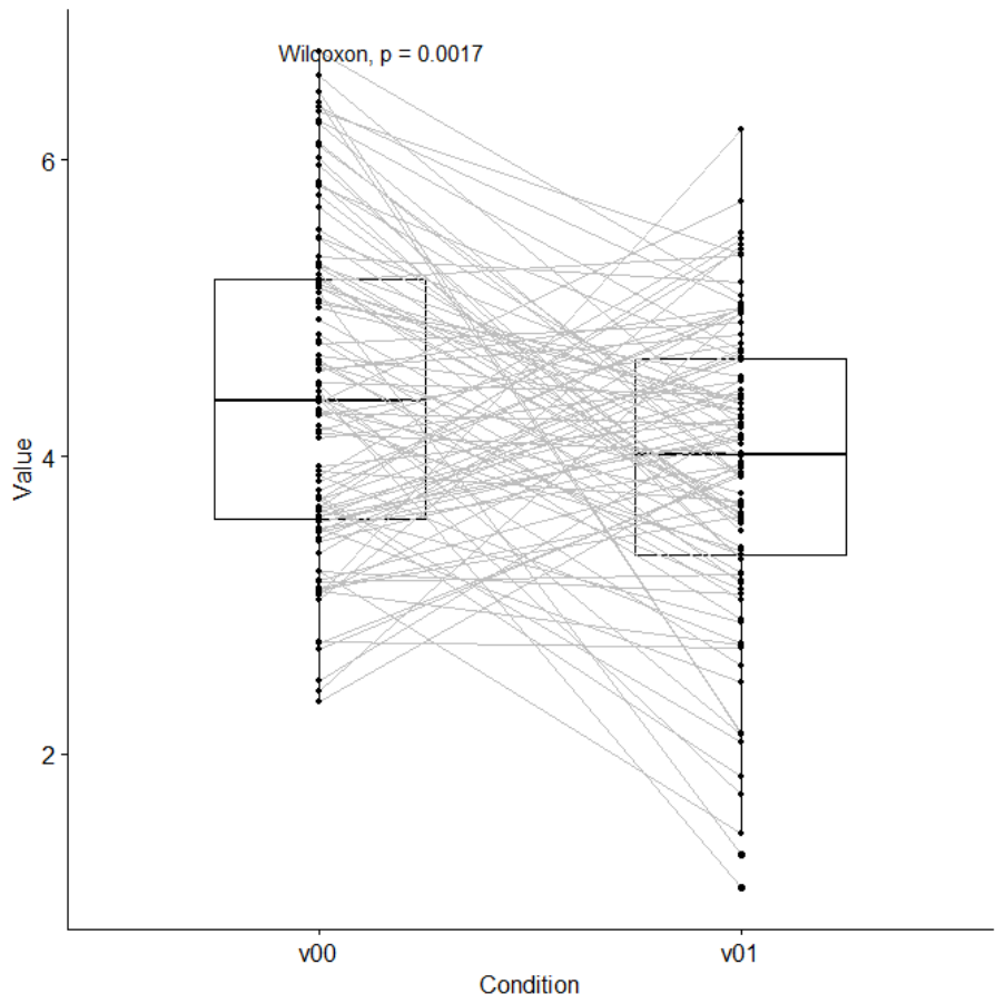
837
Figure 134. Connected boxplots for condition V
00
vs. V
01
.
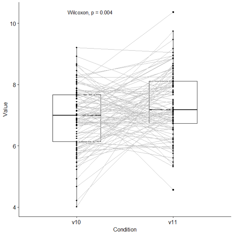
838
Figure 135. Connected boxplots for condition V
10
vs. V
11
.
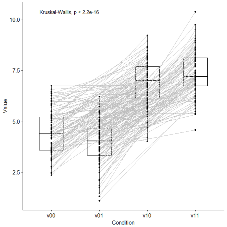
839
Figure 136. Connected boxplots for condition V
00
, V
01
, V
10
, V
11
.
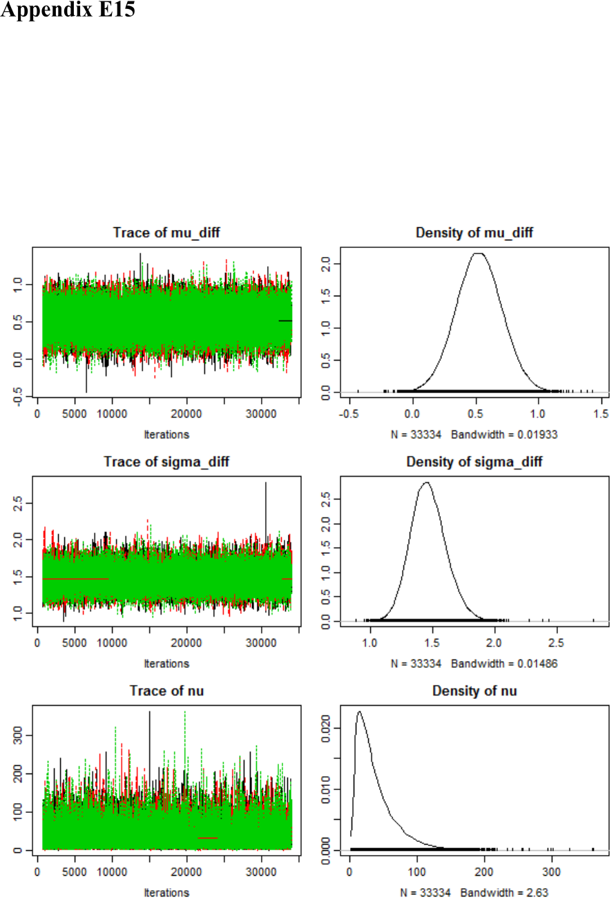
840
MCMC convergence diagnostic
This appendix contains the MCMC convergence diagnostic (i.e., ESS and MCSE) for
all parameters. The graphics show the trace plot, autocorrelation plot, shrink factor plot,
and the density plot.
V
00
vs. V
01
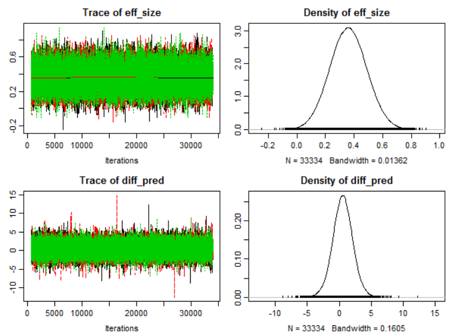
841

842
Iterations = 601:33934
Thinning interval = 1
Number of chains = 3
Sample size per chain = 33334
Diagnostic measures
mean sd mcmc_se n_eff Rhat
mu_diff -0.484 0.170 0.001 64751 1.000
sigma_diff 1.359 0.137 0.001 40827 1.000
nu 35.203 29.187 0.219 17750 1.001
eff_size -0.360 0.131 0.001 60239 1.000
diff_pred -0.482 1.468 0.005 99761 1.000
mcmc_se: the estimated standard error of the MCMC approximation of the
mean.
n_eff: a crude measure of effective MCMC sample size.
Rhat: the potential scale reduction factor (at convergence, Rhat=1).
Model parameters and generated quantities
mu_diff: the mean pairwise difference between dataexp2$v10 and dataexp
2$v11
sigma_diff: the scale of the pairwise difference, a consistent
estimate of SD when nu is large.
nu: the degrees-of-freedom for the t distribution fitted to the pairwi
se difference
eff_size: the effect size calculated as (mu_diff - 0) / sigma_diff
diff_pred: predicted distribution for a new datapoint generated
as the pairwise difference between dataexp2$v10 and dataexp2$v11

843
Quantiles
q2.5% q25% median q75% q97.5%
mu_diff 0.167 0.402 0.523 0.646 0.885
sigma_diff 1.204 1.369 1.459 1.556 1.765
nu 5.933 16.357 28.903 49.607 116.042
eff_size 0.111 0.274 0.360 0.447 0.615
diff_pred -2.596 -0.489 0.529 1.540 3.647
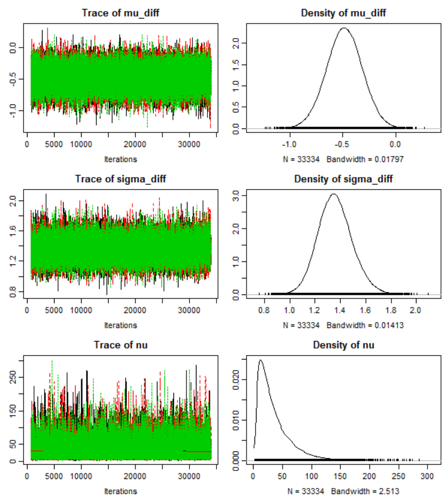
844
V
10
vs. V
11
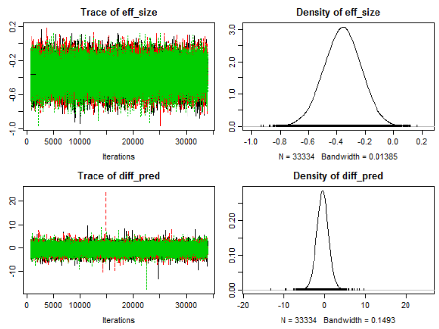
845

846
Iterations = 601:33934
Thinning interval = 1
Number of chains = 3
Sample size per chain = 33334
Diagnostic measures
mean sd mcmc_se n_eff Rhat
mu_diff 0.524 0.182 0.001 65510 1.000
sigma_diff 1.466 0.143 0.001 45218 1.000
nu 37.497 29.840 0.214 19470 1.001
eff_size 0.361 0.129 0.001 65616 1.000
diff_pred 0.529 1.571 0.005 100633 1.000
mcmc_se: the estimated standard error of the MCMC approximation of the
mean.
n_eff: a crude measure of effective MCMC sample size.
Rhat: the potential scale reduction factor (at convergence, Rhat=1).

847
Quantiles
q2.5% q25% median q75% q97.5%
mu_diff -0.821 -0.597 -0.484 -0.370 -0.152
sigma_diff 1.104 1.267 1.354 1.445 1.644
nu 5.267 14.731 26.577 46.496 112.993
eff_size -0.621 -0.447 -0.358 -0.271 -0.108
diff_pred -3.360 -1.432 -0.482 0.455 2.426
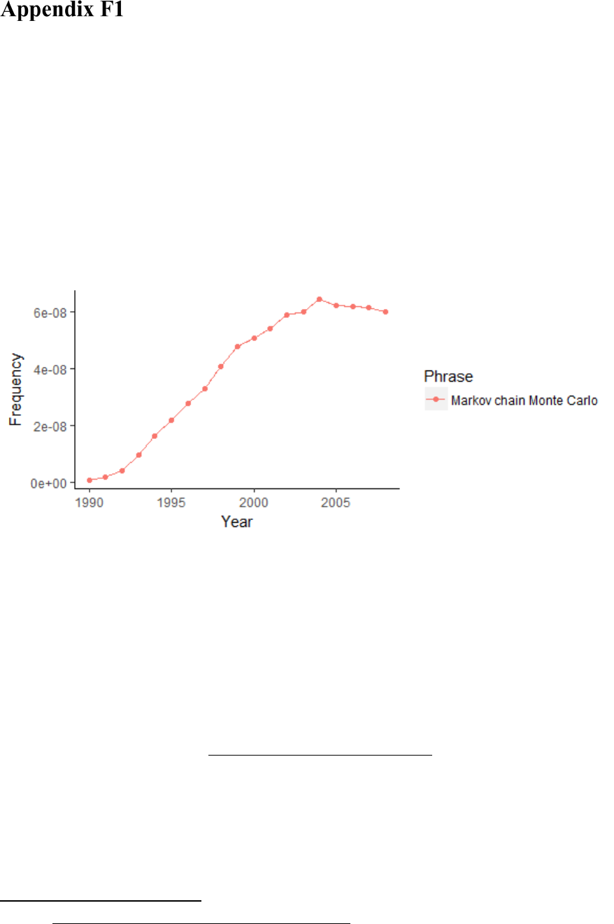
848
Appendix F Discussion
Extrapolation of methodological/statistical
future trends based on large data corpora
Bayesian Markov chain Monte Carlo sampling has gained in popularity. However, it
has been argued that the relationship between Bayesian methods and various
bootstrapping approaches is poorly understood, despite the growing use of posterior
probabilities. Moreover, simulation studies in the field of phylogenetics indicate that
their results do not always converge (Clyde & Lee, 2001).
Figure 137. Graph indicating the increasing popularity of MCMC methods since 1990.
Data was extracted from the Google Books Ngram Corpus (Lin et al., 2012) with the R
package “ngramr”.
264
Based on their aggregated data, Google developed a program to successfully predict and
“nowcast” the outbreak of flu (https://www.google.org/flutrends) by using a linear
model to compute the log-odds for the outbreak of various influenza-type viruses.
GoogleTrends is also a powerful tool to investigate the evolution (spreading, fitness) of
264
URL: https://cran.r-project.org/src/contrib/Archive/ngramr/

849
memes. The (big) data is publicly available and can be freely downloaded from the
Google servers. We argue that GoogleTrends is not only useful to make predictions
about economics (Choi & Varian, 2012; Preis, Moat, & Eugene Stanley, 2013), disease
outbreaks (i.e., epidemiological research) (Carneiro & Mylonakis, 2009; Nuti et al.,
2014), house prices (Wu & Brynjolfsson, 2009), claims for unemployment benefits
(Choi & Varian, 2009), developments in engineering (Rech, 2007), and liquidity in
German stocks (Bank, Larch, & Peter, 2011), to name just the most salient query
categories. It can also be utilised to extrapolate and forecast trends about the usage and
popularity (memetic evolution) of statistical and analytical methods. We compared
various statistical methods on the basis of dataset provided by Google. For this purpose,
we utilised the R package “gtrendsR”
265
in order to download and analyse the data.
We plotted the trends for various countries (using ISO3166-2 country codes), viz., we
visualised interest as a function f of time t (see Figure 138). A zoomable vector graphic
for closer visual inspection can be downloaded as a PDF from the following URL:
http://irrational-decisions.com/phd-thesis/gtrends-mcmc.pdf. The underlying dataset is
also available as a raw *.txt file: http://irrational-decisions.com/phd-thesis/gtrends-
mcmc.txt.
265
The code is available on the GitHub repository: https://github.com/PMassicotte/gtrendsR (the package
also allows to analyse and forecast trends for Google image searches and YouTube, Froogle, and Google
News, inter alia).
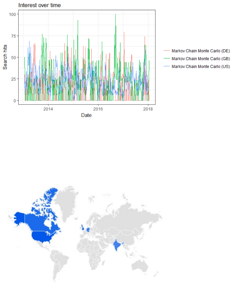
850
Figure 138. Discrete time series for the hypertext web search query “Markov chain
Monte Carlo” since the beginning of GoogleTrends in 2013/2014 for various countries
(DE=Germany, GB=Great Britain, US=United States).
Figure 139. Color-coded geographical map for the query “Markov chain Monte Carlo”
(interest by region).
If desired, the “gtrendR” package allows for much finer grained geographical analysis
(e.g., one can specifically focus on predefined cities).
851
Annex 1
N,N-Dimethyltryptamine: An endogenous
neurotransmitter with extraordinary effects.
Introduction
What is mind? No matter.
What is matter? Never mind.
--George Berkeley (1685-1753)
In this classic couplet, Bishop Berkeley concisely addressed the quintessential
philosophical question concerning the fundamental relationship between mind and
matter (note that he employs Cartesian dualistic terminology; i.e., res extensa vs. res
cogitans).
The question Berkley poses is the following: Can mind/consciousness ultimately be
explained in a purely materialistic framework (is “it” reducible to neurobiological
mechanisms, molecules, atoms, etc. pp.)? Vice versa, the quote addresses the inverse
question: Can the totality of physical reality (in Lockeian nomenclature, the entirety of
“primary and secondary qualities”) be accounted for solely in terms of mind? In other
terms, is the material world an idealistic creation of the mind, as many ancient eastern
metaphysical wisdom traditions postulate (experience, then, is the sole reality and the
observer/subject and the observed/object are of identical nature; e.g., Bhagavad Gītā,
Vedānta, Rigvedas, Yoga Sūtras of Patañjali)? This paradoxical conundrum is a deep-
rooted perennial problem in the philosophy of mind and it has recently become a topic
of interest for many neuroscientists.
852
Neurochemistry of cognition
Contemporary materialistic reductionist neuroscience emanates from the provisional
working hypothesis that the underpinnings of human cognition, perception, and
consciousness are electrochemical. That is, electrical action potentials and chemical
neurotransmission are hypothesized to ontologically cause these phenomena. However,
it is possible that this unproven assumption might eventually turn out to be a case of
epistemological naiveté.
Nevertheless, it is an established scientific fact that there are certain classes of material
substances that affect consciousness reliably (the terms consciousness and mind are
consequently used synonymously). However, not any arbitrary substance can alter the
mind. The mind-altering substances in question have precisely defined molecular
structures, which in turn cause very specific effects. For instance, there are certain
psychoactive substances that induce sedation (for instance, Diazepam). This particular
sedative is a specific case of a much larger chemical class (i.e., the Benzodiazepine
family). Thus, there appears to be a systematic correlation between the chemical
structure of certain compounds and the psychological effects they induce (in
psychopharmacology this is known as the structure-activity relationship).
Interestingly, especially from a neurochemistry/biology point of view, several naturally
occurring secondary (possibly semiotic) plant compounds have close structural
relationships with various mammalian (including human) neurotransmitters and can
consequently bind to specific cell membrane receptors in the brain. Thereby, these
chemicals can reliably change a variety of cognitive and perceptual processes (both
quantitatively and qualitatively). N,N-Dimethyltryptamine (abbreviated as DMT) is a
prototypical exemplar of such psychoactive chemicals (DMT has been oxymoronically
referred to as “the spirit molecule”; but see Strassman, 2001). The receptor binding
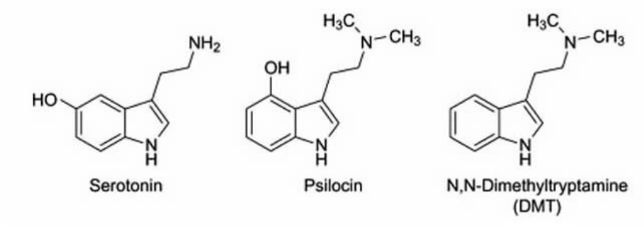
853
affinity of DMT is complex and hitherto only partially understood. However, it has been
firmly established that DMT non-selectively agonises several members of the 5-HT
2
(5-
hydroxytryptamin also known as Serotonin) receptor family (especially the 5-HT
2A
and
5-HT
2B
receptor appear to be crucial for its psychoactive effects; but see McKenna et
al., 1990; Aghajanian & Marek, 1999; Keiser et al., 2009). Except for the 5-HT
3
receptor, all 5-HT receptors achieve transmembrane signal transduction via the G-
protein-coupled receptors. Recently, important fundamental research on the G protein-
coupled receptor led to a series of Nobel Prizes (e.g., in 2000, 2004, and 2012).
Moreover, it has recently been demonstrated that DMT is an endogenous σ
1
receptor
regulator (Fontanilla et al., 2009;) and it has been hypothesized that it plays a mediative
role in tissue protection, regeneration, and immunity (Frecska et al., 2013). From a
chemical point of view, DMT is a prototypical representative member of the
indolealkylamine family known as tryptamines. In its pure form, DMT is a white/clear,
pungent-smelling, crystalline solid. Its molecular structural geometry visualized in
Figure 140 is closely related to Serotonin.
Figure 140. Chemical structures of Serotonin, Psilocin, and N,N-Dimethyltryptamine in
comparison.
854
Compounds such as psilocin (synonymous with 4-hydroxy-N,N-dimethyltryptamine, a
precursor of psilocybin which is also known as O-phosphoryl-4-hydroxy-N,N-
dimethyltryptamine) and DMT (N,N-Dimethyltryptamine) have chemical structures that
resemble the neurotransmitter serotonin (5-hydroxytryptamine). This structural
similarity to serotonin allows them to stimulate serotonin-sensitive neurons. Note that
the intermolecular serotonin motif is embedded in both structures.
From a phylogenetic perspective, DMT is an evolutionary very old molecule which is
ubiquitously present in the plant and animal kingdom (Smith, 1977). In 1961, Nobel
Prize laureate Julius Axelrod reported in the journal Science that the enzyme N-
methyltransferase in a rabbit's lung is able to mediate the biotransformation of
tryptamine into DMT (Axelrod, 1961). More recent converging evidence strongly
suggests that DMT is an endogenous neurotransmitter in the human brain (e.g., Cozzi,
et al., 2011; Fontanilla, et al., 2009; Cozzi, et al., 2009). Surprisingly, DMT is actively
transported into the brain via the blood-brain-barrier (a process that is costly in
energetic terms because it requires movement against the concentration gradient). This
factum has been discovered by Japanese scientists 30 years ago (i.e., Yanai et al., 1986).
Given that the brain in an extremely sensitive homeostatic organ, it constantly protects
itself from toxins and undesired agents. Consequently, the blood-brain-barrier is highly
selective and only very few essential compounds like glucose and other essential
nutrients are actively moved across this membrane into the brains tissue. The
phenomenon that DMT is actively transported across this protective barrier suggests
that it plays a crucial role in ordinary brain metabolism. Moreover, DMT does not built
up tolerance, as other psychoactive tryptamines do (no significant desensitisation after
repeated administration; see Strassman & Qualls, 1994; Strassman et al., 1994) and it is
855
quickly metabolised (consequently its duration of action is relatively short-lived) .
Again, this indicates that it is a natural building block of mammalian neurochemistry.
At the moment, there is no explanation as to why mammals have evolved an
endogenous neurotransmitter that is able to produce profoundly altered states of
consciousness. From an evolutionary point of view one has to ask the question: What is
the adaptive advantage of this compound in terms of survival or reproduction?
However, given that the intracellular cascade triggered by DMT is not yet fully
understood it seems very difficult to imagine that science is soon able to account for its
much more intricate effects on perception and consciousness (the hard problem) from a
quantitative point of view.
DMTs qualitative phenomenology
From a psychological vantage point, DMT has very remarkable effects, too. One of
DMTs most salient activity characteristics is that it affects visual perception in the most
spectacular ways possibly imaginable. In addition, it profoundly changes the
functioning of a multitude of core cognitive capacities. A brief (though incomplete)
synopsis of DMTs subjective effects is summarised in the following list:
• Profound changes in sensory perception across modalities (e.g., perceptual
distortions, vivid cross-modal hallucinations, visions, synaesthesia)
• Highly symmetric and oftentimes fractal multidimensional visual hallucinations of
astonishing beauty and complexity
• Spectacular visual percepts (impossible objects which are essentially ineffable)
• Subjective experience of extrasensory perceptions (e.g., telepathic phenomena are
commonly reported)
856
• Changes in time and space perception (e.g., time dilation, timelessness/experience
of infinity/eternity, limitlessness/omnipresence)
• Journey-like “breakthrough into hyperspace” (trans-dimensional travel into parallel
dimension and contact with conscious “otherworldly humanoid beings” is
commonly reported under high doses of DMT)
• Altered body image (e.g., out-of-body-experience, taking on an animal/alien body)
• Intense changes in mood (ranging across the whole spectrum of emotions from total
serenity/bliss to extreme terror)
• Sense of profound meaning and deep spiritual insights (e.g., gnosis)
• Experience of very profound “mystical states”
• Dissolution of ego boundaries (e.g., ego-death, shared consciousness)
• Feelings of interconnectedness (e.g., communion with nature, monistic all-is-one
experience)
• State of union and spontaneous realisation of oneness (nonduality, yoga)
• Near-death experience
• Experience of emptiness, nothingness, pure I-am-ness
• Feelings of tranquillity
• Being freed from one’s body and becoming integrated with one’s cosmic nature
• Feeling of sudden realisation of one’s homogenous cosmic essence
• State of inner harmony (Samādhi)
• Experience of a transcendental reality
• Collapse of ego-ignorance phantom (dissolution of self-limitation)
• Transformation of self-perception, transmutation of entire being (self-
transcendence)
• Expansion of awareness (experience of boundless primordial awareness)

857
• Experience of higher states of consciousness
• Feelings of awe and wonder
• Feeling of awakening from an illusion to a larger “more real” reality
• Appreciation of nature (perception of nature as animated and alive, biophilia)
• Sudden insights into the nature of self and the nature of reality (epiphany or “satori”
like experience - seeing into one's true nature)
• Access to unconscious “Jungian alchemical archetypal” information
Potential adverse effects
• Acute panic reaction (depending on idiosyncratic personality structure and situation)
• Substance induced psychosis (ICD-10 diagnosis code F16.5 – low incidence rate)
• Hallucinogen persisting perception disorder (DSM-IV diagnosis code 292.89 – low
incidence rate)
The following paragraphs reprint two experiences reported by research subjects who
participated in Rick Strassmans early DMT which were conducted in Mexico in the
1990s.
“The trip started with an electric tingling in my body, and quickly the visual
hallucinations arrived. Then I noticed five or six figures walking rapidly alongside me.
They felt like helpers, fellow travelers. A humanoid male figure turned toward me,
threw his right arm up toward the patchwork of bright colors, and asked, "How about
this?" The kaleidoscopic patterns immediately became brighter and moved more
rapidly. A second and then a third asked and did the same thing. At that point, I decided
to go further, deeper. I immediately saw a bright yellow-white light directly in front of
me. I chose to open to it. I was consumed by it and became part of it. There were no
distinctions—no figures or lines, shadows or outlines. There was no body or anything
858
inside or outside. I was devoid of self, of thought, of time, of space, of a sense of
separateness or ego, or of anything but the white light. There are no symbols in my
language that can begin to describe that sense of pure being, oneness, and ecstasy.
There was a great sense of stillness and ecstasy.” (excerpt taken from Strassman, 2001;
p.244)
“Eight minutes into his non-blind high-dose injection, he described this encounter:
That was real strange. There were a lot of elves. They were prankish, ornery, maybe
four of them appeared at the side of a stretch of interstate highway I travel regularly.
They commanded the scene, it was their terrain! They were about my height. They held
up placards, showing me these incredibly beautiful, complex, swirling geometric scenes
in them. One of them made it impossible for me to move. There was no issue of control;
they were totally in control. They wanted me to look! I heard a giggling sound - the
elves laughing or talking at high-speed volume, chattering, twittering.” (excerpt taken
from Strassman, 2001, p. 188).
It should be noted that the phenomenological experiences reported under the influence
of DMT are interindividually very heterogeneous (perhaps partially due to a
combination of genetically coded neurotransmitter receptor polymorphisms and
idiosyncratic psychological variables) and are contingent upon set and setting (that is,
internal psychological and external situational factors play an important role). However,
several phenomenologies are reliably induced across diverse subjects (e.g., complex
visual hallucinations, out-of-body-experiences, trans-dimensional travels, etc.).
Space does not permit a detailed discussion of DMTs experiential phenomenology,
particularly because linguistic expressions are circuitous and often largely inadequate in
order to convey its diverse spectrum of psychological effects (ineffability is a defining

859
hallmark of the translinguistic DMT ontology which reaches far beyond the bounds of
human imagination). The perceptions and insights that are catalysed by this compound
are often described as being at total invariance with the socially grounded models of
contemporary western paradigms. Interestingly, several of DMTs structural analogues
(e.g., Psilocybin, a compound which is present in the “magic” mushrooms which are
endemic to the UK, Mantle & Waight, 1969; see also Figure 1) have
phenomenologically comparable though not identical effects (cf. Hasler et al., 2004).
However, hitherto the extraordinary cognitive changes triggered by DMT cannot be
accounted for by any of the existing theoretical frameworks provided by neuroscience
and psychology.
Endogenous but prohibited
Despite the exceptional characteristics of DMT and its ubiquity in nature, many
mainstream psychologists and even professional neuroscientists are utterly unaware of
its existence (presumably, due to academic overspecialisation and the fact that the
conventional neuroscience textbooks do not mention it at all, e.g., Gazzaniga &
Mangun, 2014; Kolb & Whishaw, 2009). Furthermore, systematic and methodologically
valid research is highly restricted due to the fact that DMT is classified as a “Class A
drug” in the UK and similarly tightly regulated as a “Schedule I substance” in the US.
This classification is clearly not evidence based and it inhibits scientific progress and
innovation (let alone the fact that it violates the principle of cognitive liberty, that is, the
right to mental self-determination).
In this context, it is noteworthy that the Brazilian União do Vegetal (UDV -
www.udv.org.br) was granted precedential legal permission to use a DMT containing
drink (named Ayahuasca) in their ceremonies. The UDV, which is claiming roots as far
860
back as the 10
th
century BC, utilises Ayahuasca in a program of spiritual evolution
based on mental concentration and the search for self-knowledge. From a juridical point
of view, it is very interesting that the US Supreme Court adjudicated in 2006 that the
UDV is legally permitted to deploy Ayahuasca as a religious sacrament (under the
protection of the “Religious Freedom Restoration Act”).
Ayahuasca: An ancient phytochemical synergy
From a much larger historical perspective, DMT has been utilized for
spiritual/shamanistic rituals for millennia by several ancient cultural traditions. As
mentioned before, it constitutes the active pharmacological principle in Ayahuasca, a
plant based, drinkable concoction, which is traditionally used by indigenous tribes in the
Amazonian rainforest for divinatory and healing purposes. In itself, DMT is orally
inactive because the monoamine oxidase (MAO) system within the gastro-intestinal
(GI) tract deaminates it. However, somehow the aboriginals have developed
sophisticated intuitive knowledge concerning its combinatorial pharmacodynamics. In
order to prevent DMTs decomposition in the gut, they mix it with a plant-based MAO
inhibitor.
To be specific, the typical primary ingredients of the Ayahuasca brew consist of two
plants, Psychotria Viridis (which contains the DMT) and Banisteriopsis Caapi (which
contains the β-carboline harmala alkaloid designated as harmine). Harmine functions as
a selective and reversible inhibitors of the enzyme monoamine oxidase A (MAO-A) that
prevents the enzymatic breakdown of DMT in the GI-tract, thereby allowing it to be
transported via the blood-brain barrier. Hence, it is the combination of these two plants,
which enables DMT to become psychoactive. Quite thought-provokingly, the chemical
literature labelled Harmine for some time as telepathine. This chemical was so named
861
because of the effects reported by Amazonian tribal members (e.g., telepathic
communication, clairvoyance, precognition, psychic diagnosis, necromancy).
Western science has just relatively recently learned about DMT and its psychoactive
effects from ethnophamacologists who were able to conserve this ancient cultural
knowledge literally in the last minute because old shamanic traditions are being
extinguished at a fast pace by the modern industrial world. The inhabitants of the
Amazonian rainforest have a very close relationship with, what they call “plant-spirits”.
They regard Ayahuasca as a wise “plant teacher” which enables them to communicate
with the “spirit world” (Beyer, 2009). It should be noted that in the shamanic paradigm
the dichotomy between spiritual and medicinal is not clear-cut as the European heritage
suggests and “sacred” plants play a central role in these traditional indigenous contexts.
Unfortunately, the Amazonian rainforests are currently being destroyed at a very
alarming rate. The Amazonian biodiversity is among the richest in the world, although
the number of species in the red list of the IUCN (International Union for Conservation
of Nature) is growing steadily every year. The destruction of the natural environment
goes hand in hand with the loss of culturally embedded ancient folk-knowledge
concerning the utilisation of specific plants for medicinal and spiritual purposes.
Moreover, younger generations are not very interested in the continuation of the
Shamanic traditions of their predecessors. They prefer to move into modern
technologized cities in order to take their place in the materialistic market economy and
consequently thousands of years of accumulated and potentially highly valuable
information is lost in this cultural transition.
Conclusion
862
Brevity does not permit me to review many intriguing aspects of this multifaceted topic
(e.g., DMTs relation to psychological conditioning/extinction, neurogenesis,
neuroplasticity, psychoneuroindocrinology, psychoimmunology, epigenetics, and the
neuroanatomical correlates of its effects). I could only try to provide a very rudimentary
introduction to this fascinating newly emerging research domain. It should be
emphasized that this subject (psychoactive plant compounds and human cognition,
perception, and consciousness) is located at the cutting edge of modern cognitive
neuroscience and psychology and it encompasses many other adjacent disciplines (e.g.,
physics, chemistry, botany, pharmacology, psychiatry, anthropology, history,
archaeology, philosophy, religion, medicine, art, law, ethics, etc. pp.; cf. Bois-Mariage,
2002).). I am convinced that many researchers will develop a deep interest for this topic
if they have not already done so.
For further information, the interested reader is referred to the book “DMT: The spirit
molecule” by Rick Strassman (2001) who was the first to conduct FDA approved
rigorous scientific human trials with DMT in the 1990s. His book provides a
comprehensive synopsis of DMTs neurochemistry and its experiential phenomenology.
Strassman hypothesized back in the 90s that DMT might be present in the human pineal
gland. This hypothesis was largely ignored by the scientific community. However, his
prediction has recently been partially corroborated. In 2013, researchers first reported
the presence of DMT in rodent pineal gland microdialysate (Barker, et al., 2013). The
pineal is a photoreceptive endocrine gland whose primarily known function is the
regulation of the circadian rhythm via the secretion of melatonin (N-acetyl-5-methoxy
tryptamine), another serotonergic member of the tryptamine family (but see Reiter,
1991). Because the photosensitive pinealocytes have a strong resemblance to the
photoreceptor cells of the eye, the pineal gland has also been labelled as the “third

863
parietal eye” (Eakin, 1973). It has been subject to much speculation since Claudius
Galenus and later René Descartes who famously termed it the “principal seat of the
soul”.
Future research directions
To conclude, I would like to delineate some potentially fruitful directions for future
research on DMT and formulate several empirically testable hypotheses:
DMT and its vastly more potent relatives (e.g., 5-methoxy-N,N-dimethyltryptamine
acronymized as 5-Meo-DMT) might lead to the discovery of new classes of
neurotransmitter systems (cf. the discovery of the endocannabinoid system) that would
deepen our understanding of basic neurochemistry and may ultimately lead to the
design of new pharmacological agents in order to treat mental pathologies (cf. Jacob &
Presti, 2005) or to enhance cognition (e.g., nootropics) or expand consciousness in the
healthy population.
Another research agenda should focus the role of DMT and its relatives in molecular
biology. The National Genome Research Institute published data that indicates that the
costs of genetic sequencing (DNA micro arrays) are decreasing fast than Moore’s law
for computational performance predicts (http://genome.gov/sequencingcosts). This
development opens up unprecedented large-scale analytic possibilities for the newly
emerging discipline of neurogenetics. For example, in analogy to the genome, the
proteome, and the connectome, the receptorome aims to map the total number of genes
that code for receptors and receptor molecules in the brain. In this regard, it has recently
been argued in a paper titled “Psychedelics and the Human Receptorome” that “it
should be possible to use this diverse set of drugs (psychedelics) as probes into the roles
864
played by the various receptor systems in the human mind” (Ray, 2010, p.1; content in
bracket added).
The neurochemical correlates of the various meditative states of mind are another
vibrant research topic. Researchers have observed statistically significant overlap
between the neural correlates of mediation and psychedelic experiences. Consequently,
there might be a significant degree of overlap between the neurochemical substrates of
these altered states of mind. In this regards, the influence of DMT on microtubule
(neuronal microstructures which form part of the cytoskeleton) should be a focal point
of systematic scrutiny (but see Hameroff & Penrose, 2014).
Recent research provides evidence that DMT has psychoneuroendocrinological and
psychoneuroimmunological effects (Frecska et al., 2023). Fascinatingly, it has been
shown in a publication by Epel et al. in 2009 (co-authored by Nobel Prize laureate
Elizabeth Blackburn) that mediation influences telomere length (an indicator of
biological age). Given that DMT and various related psychoactive tryptaminergic
compounds induce states of mind that are partially qualitatively congruent with the
mental states achieved by meditative practices it seems likely that the experiences
triggered by DMT also have the potential to positively affect telomere length (e.g., via
telomerase activity). Based on the assumption that DMT can induce robust longitudinal
changes on various levels (physical and psychological) it seems likely that genetic
changes are involved. Future research should focus on the (epi)genetic fundament of
these changes (how gene methylation/transcription/ expression is altered following
exposure to psychoactive substances).
Another line of research should investigate the interplay between quantum physical
phenomena and altered states of consciousness. The theoretical framework of quantum
865
physics ascribes a pivotal role to consciousness (e.g., Schrödinger's wave equation).
Consequently, substances which profoundly change the main pillar of this theoretical
tenet (that is, consciousness and the associated mechanics of perception) should be of
significant interest to the physics community. The disciplines of physics and
psychology should pursue a close interdisciplinary discourse and collaborations in order
to combine their efforts and insights (this has happened before, for instance, the
physicists Albert Einstein and Wolfgang Pauli were in close communication with depth-
psychologist C.G. Jung).
Yet another auspicious line of research is an investigation of the effects of DMT on
creative thinking and cognitive flexibility (i.e., DMT as a catalyst for creativity and
innovation; cf. Frecska et al., 2012). Given that DMTs phenomenology deconstructs
conventional orthodox cultural worldviews it has the potential to facilitate novel
perspectives on multifarious philosophical questions and might even contribute to the
resolution of “hard” scientific problems (cf. Willis, et al., 1966).
There is much more scientific virgin soil that awaits thorough investigation. A largely
unexploited research area comprises of careful empirical tracings of the effects of
various non-naturally occurring synthetic psychoactive tryptamines which have been
developed by the pioneering chemist Alexander Shulgin (see Shulgin & Shulgin, 1997).
His work entails an extensive chemical toolbox for future work in neuroscience and
psychology. In his book “TiHKAL - Tryptamines I have known and loved” he provides
a detailed index of more than 50 psychedelic compounds (many developed by himself).
The book entails a description of their synthesis, exact chemical structures, dosage
recommendations, and qualitative comments. Most of these compounds have yet to be
rigorously researched – a task for the next generation of curious and open-minded
scientists. To provide an intriguing example, one of the tryptamines described by

866
Shulgin is DiPT (Diisopropyltryptamine). It has unique properties because it does
almost exclusively affect the auricular sense (i.e., nonlinear shifts in pitch perception -
other sensory modalities remain largely unaffected). It is apparent that DiPT should be
of keen interest to researchers trying to understand the neural basis of auditory
perception. However, up until now systematic research has not been conducted
(experimental ornithological studies of avian vocalisation/bioacoustics might be a fertile
starting point).
Finally yet importantly, the experiences DMT evokes are of particular fascination to
artists, for obviously reasons (e.g., Grey, 2012). Several visionary artists have been
deeply inspired by their transcendental experiences with DMT and related compounds
(see Figure 2).
Figure 2: The net of being by Alex Grey (inspired by the Mahayanian metaphor of
Indra's net).
Further artworks created by Alex Grey are available under the following URL:
http://alexgrey.com/art/
867
Finally, it remains an open question why DMT (and its structural relatives) are not part
of the mainstream discourse in psychology and neuroscience. Especially given its
apparently central role in perceptual processes, its pertinence for consciousness studies,
its implications for understanding mood disorders and emotions in general, and its far-
reaching philosophical implications? A Kuhnian paradigm shift is needed. The study of
naturally occurring (plant derived) substances should be allowed into academia in order
to foster the elucidation of the interplay between psychoactive chemicals, cognition, and
consciousness.
Off the Lip: Science over politics!
References
Adams, C., Waldstein, A., Luke, D., Sessa, B. & King, D. (2013). Breaking convention:
Essays on psychedelic consciousness. Devizes: Strange Attractor.
Aghajanian, G.K. & Marek, G.J. (1999). Serotonin and Hallucinogens.
Neuropharmacology, 21, 16-23.
Axelrod, J. (1961). Enzymatic formation of psychotomimetic metabolites from
normally occurring compounds. Science. 134(3475), 343.
Barker, S.A., Borjigin J., Lomnicka, I., Strassman, R. (2013). LC/MS/MS analysis of
the endogenous dimethyltryptamine hallucinogens, their precursors, and major
metabolites in rat pineal gland microdialysate. Biomedical Chromatography, 27, 1690-
1700.
Beyer, S. (2009). Singing to the plants: A guide to mestizo shamanism in the upper
Amazon. Albuquerque: University of New Mexico Press.
868
Bois-Mariage, F. (2002). Ayahuasca : Une synthèse interdisciplinaire. Psychotropes, 8,
79-113.
Cozzi, N.V., Gopalakrishnan, A., Anderson, L.L., Feih, J.T., Shulgin, A.T., Daley, P.F.,
Ruoho A.E. (2009). Dimethyltryptamine and other hallucinogenic tryptamines exhibit
substrate behavior at the serotonin uptake transporter and the vesicle monoamine
transporter. Journal of Neural Transmission, 116(12), 1591–1599.
Cozzi, N.V., Mavlyutov, T.A., Thompson, M.A., Ruoho, A.E. (2011). Indolethylamine
N-methyltransferase expression in primate nervous tissue. Society for Neuroscience
Abstracts, 37, 840.19.
Eakin, R. (1973). The third eye. Berkeley: University of California Press.
Epel, E., Daubenmier, J., Moskowitz, J. T., Folkman, S., Blackburn, E. (2009). Can
meditation slow rate of cellular aging? Cognitive stress, mindfulness, and telomeres.
Annals of the New York Academy of Sciences, 1172, 34-53.
Fisher, R.A. (1971). A cartography of the ecstatic and meditative states. Science, 174,
897-904.
Frecska, E., Móré, C.E., Vargha, A., Luna, E.L. (2012). Enhancement of Creative
Expression and Entoptic Phenomena as After-Effects of Repeated Ayahuasca
Ceremonies. Journal of Psychoactive Drugs, 44(3), 191-199.
Frecska, E., Szabo, A., Winkelman, M.J., Luna E.L. and McKenna, D.J. (2013). A
possibly sigma-1 receptor mediated role of dimethyltryptamine in tissue protection,
regeneration, and immunity. Journal of Neural Transmission, 120(9), 1295–1303.

869
Fontanilla, D., Johannessen, M., Hajipour, A.R., Cozzi, N.V., Jackson, M.B., Ruoho,
A.E. (2009). The Hallucinogen N,N-Dimethyltryptamine (DMT) Is an Endogenous
Sigma-1 Receptor Regulator. Science, 323(5916), 934-937.
Gazzaniga, M. & Mangun, G. (2014). The cognitive neurosciences. Cambridge,
Massachusetts: The MIT Press.
Grey, A. (2012). Net of being. Rochester, Vermont: Inner Traditions.
Grof, S. (2000). LSD-Psychotherapie. Stuttgart: Klett-Cotta.
Hameroff, S. & Penrose, R. (2014). Consciousness in the universe: A review of the
‘Orch OR’ theory. Physics of Life Reviews, 11(1), 39-78.
Hasler, F., Grimberg, U., Benz, M.A., Huber, T., Vollenweider, F.X. (2004). Acute
psychological and physiological effects of psilocybin in healthy humans: a double-
blind, placebo-controlled dose-effect study. Psychopharmacology, 172, 145-156.
Huxley, A. (1954, 1956). The Doors of Perception and Heaven and Hell, New York:
Harper Collins.
Jacob, M.S.& Presti, D.E. (2005) Endogenous psychoactive tryptamines reconsidered:
an anxiolytic role for dimethyltryptamine. Medical Hypotheses. 64, 930-937.
Keiser, M.J., Setola, V., Irwin, J.J., Laggner, C., Abbas, A.I., Hufeisen, S.J., Jensen,
N.H. et al. (2009). Predicting new molecular targets for known drugs. Nature,
462(7270), 175–81.
Kolb, B. & Whishaw, I. (2009). Fundamentals of human neuropsychology. New York,
NY: Worth Publishers.
870
McKenna, D.J., Repke, D.B., Lo, L., Peroutka, S.J., (1990). Differential interactions of
indolealkylamines with 5-hydroxytryptamine receptor subtypes. Neuropharmacology,
29, 193-198.
Mantle, P.G., Waight, E.S. (1969). Occurrence of psilocybin in sporophores of
Psilocybe semilanceata. Transactions of the British Mycological Society, 53(2), 302-
304.
Ray, T.S. (2010). Psychedelics and the Human Receptorome. PLoS ONE, 5(2), e9019.
Reiter, R.I. (1991). Pineal gland. Interface between photoperiodic environment and the
endocrine system. Trends in Endocrinology and Metabolism, 2(1), 13-19.
Shulgin, A. & Shulgin, A. (1997). Tihkal: The continuation. Berkeley, CA: Transform
Press.
Smith, T. (1977). Tryptamine and Related Compounds in Plants, Phytochemistry, 16,
171-175.
Strassman, R. (2001). DMT: The spirit molecule: A doctor's revolutionary research into
the biology of near-death and mystical experiences. Rochester, Vt: Park Street Press.
Strassman, R.J., Qualls, C.R. (1994). Dose-response study of N,N-dimethyltryptamine
in humans. I. Neuroendocrine, autonomic, and cardiovascular effects. Archives of
General Psychiatry, 51(2): 85-97.
Strassman, R.J., Qualls, C.R., Uhlenhuth, E.H., Kellner, R. (1994). Dose-response study
of N,N-dimethyltryptamine in humans. II. Subjective effects and preliminary results of
a new rating scale. Archives of General Psychiatry. 51(2), 98-108.
871
Harman, W.W., McKim, R.H., Mogar, R.E., Fadiman, J., Stolaroff, M.J. (1966)
Psychedelic Agents in Creative Problem-Solving: A Pilot Study. Psychological Reports.
19, 211-27.
Yanai, K., Ido, T., Ishiwata, K., Hatazawa, J., Takahashi, T., Iwata, R., Matsuzawa, T.
(1986). In vivo kinetics and displacement study of a carbon-11-labeled hallucinogen, N,
N-[11C]dimethyltryptamine. European Journal of Nuclear Medicine. 12, 141-146.
872
Annex 2
5-methoxy-N,N-dimethyltryptamine: An ego-
dissolving catalyst of creativity?
Abstract
5-MeO-DMT is an endogenous tryptamine alkaloid with a high, nonselective affinity
for various serotonin receptors. It has a unique psychopharmacological profile and its
effect cannot be compared to other psychedelics. Despite it wide distribution in nature
and long history of human usage, systematic psychological research is currently
virtually absent. We argue for the utility of various naturally occurring serotonergic
psychoactive compounds as valuable psychological research tools which have the
potential to advance our understanding of cognitive and neuronal processes, especially
those which underpin various aspects of creativity and aesthetic perception. We
postulate that 5-MeO-DMT has great scientific merit in this respect due to its
unparalleled ego-dissolving properties. An eclectic interdisciplinary perspective is
adopted, and we present ethnographic, historical, qualitative, and quantitative evidence
in support of our claim. The article then reviews two pertinent recent empirical
experimental studies in more detail: 1) A psychopharmacological study focusing on the
role of psilocybin on the Big-5 personality trait "Openness to Experience" and 2) a
multimodal fMRI based cognitive neuroscience study which investigates the influence
of LSD on neuronal functional connectivity patterns. Based on this empirical and
theoretical background, we formulate several novel and experimental falsifiable
hypotheses concerning the role of 5-MeO-DMT as a neurochemical catalyst of
creativity. Finally, we briefly adumbrate the de facto irrational "quasi-Orwellian" nature
of the recently ratified "Psychoactive Substances Act" (2016, United Kingdom) which
873
inhibits systematic scientific research, antagonizes neurodiversity, and presents a
juridically unjustifiable violation of the unalienable human right to cognitive liberty
(i.e., freedom of thought). The implications of this highly restrictive and non-evidence
based legal framework for unbiased systematic scientific research will be discussed
from a Jamesian radical empiricism perspective. In line with other creativity researchers
(e.g., Puccio, 2017), we argue that creativity plays a crucial role for the seriously
endangered survival of the species and that it is therefore of immense importance to
foster novel ways of perceiving, thinking, and consequently behaving.

874
Introduction
The following quotation from Abraham Maslow’s book “Towards a psychology of
being” provides an apt primer and some grounding for the following discussion:
“An essential aspect of SA [Self-Actualized] creativeness was a special kind of
perceptiveness that is exemplified by the child in the fable who saw that the king had no
clothes on - this too contradicts the notion of creativity as products. Such people can
see the fresh, the raw, the concrete, the ideographic, as well as the generic, the abstract,
the rubricized, the categorized and the classified. Consequently, they live far more in
the real world of nature than in the verbalized world of concepts, abstractions,
expectations, beliefs and stereotypes that most people confuse with the real world. This
is well expressed in [Carl] Rogers' phrase "openness to experience" (Maslow, 1968, p.
145, contents in brackets added by the author).
The “single-state fallacy” (T. B. Roberts, 2006, p. 104) pertains to the widely held naïve
assumption that worthwhile cognition exclusively takes place in “normal” alert waking
consciousness. However, there exists copious evidence that important creative ideas can
emerge from non-ordinary states of mind (Tart, 1972, 2008). A well-documented
illustrative historical example is August Kekulés discovery of the benzene structure in
1858, a landmark in the history of science which heralded the birth of the structural
theory of organic chemistry (Kekulé, 1866, 1890). Kekulé had a daydream of the
Ouroboros (an ancient symbol of a snake seizing its own tail) and this dream-image
provided him with the idea of the cyclic structure of benzene (Rocke, 2015).
Interestingly, the depth-psychologist C.G. Jung assigned specific archetypal and
alchemical significance to this symbol (Jung, 1969).

875
Jung’s mentor, Sigmund Freud, regarded dreams as the royal road to the unconscious
(Freud, 1939). However, unbeknownst to Freud, besides dreams and free-association
techniques there are other much more effective methods that can make unconscious
contents more accessible. Certain neuroactive chemical substances, colloquially termed
psychedelics, are particularly productive tools in this regard. There is significant
evidence that psychedelics can, inter alia, enhance creative ideation (e.g.,
ideoplasticity)
266
and aesthetic perception.
Numerous self-reports indicate that psychedelics facilitate perspectival multiplicity. In
the context of creative problem-solving, it has been suggested that psychedelics can
enable the adoption of “multiple viewpoints of a problem” (Sessa, 2008). In other
terms, a larger proportion of the entire solution space is simultaneously taken into
consideration
267
. Psychedelics have the potential to facilitate the cognitive ability to
handle multiple seemingly paradoxical alternatives simultaneously, i.e., their
neurochemical effects assist the cogniser to overcome the need for closure and they
facilitate the ability to deal with contextual ambiguity and vagueness, concepts which
are interestingly of crucial importance in the context of non-Kolmogorovian quantum
logic (Blutner et al., 2013; Putnam, 1983). We argue that psychedelics soften the
rigidity of habitual cognitive structures, thereby enabling novel and more flexible
modes of cognition
268
. For instance, the third Aristotelian law of thought (tertium non
datur), i.e., the law of the excluded middle (Whitehead & Russell, 1910), can be more
266
The term “ideagens” has been suggested (T. B. Roberts, 2006).
267
The underlying cognitive and neural mechanism are hitherto not well-understood but potential
functional models involve Baddeley’s model of working memory (e.g., visuospatial sketchpad,
excecutive functions; Baddeley, 1992). Associated neuroanatomical correlates likely involve
prefrontal/cingulate/limbic structures (Della Sala, Gray, Spinnler, & Trivelli, 1998; Kerns et al., 2004;
Madarasz et al., 2016). From a neurochemical point of view, the various serotonergic neurotransmitter
systems appear to be of central importance (Carhart-Harris & Nutt, 2017; Meneses, 1999; Nichols, 2016).
268
Experimental research on the effect of various psychedelics on functional fixedness would be
potentially fruitful to empirically corroborate this postulate. It has been argued that “innovation relies on
the obscure” and that the overcoming functional fixedness is crucial in this respect.

876
readily transcended and multiple seemingly polar (paradoxical) propositions can be held
simultaneously thereby multiplying cognitive degrees of freedom (e.g., in the context of
combinatorial/divergent thinking). The quantum physical concept of complementarity
appears to be pertinent in this respect
269
. These epistemological aspects of the
psychedelic experience might also prove to be of central importance for the psychology
of thinking and reasoning (for instance, in the context of Kahneman and Tversky’s
heuristics and biases research tradition). For instance, psychedelics might help to
overcome certain cognitive biases, e.g., self-serving confirmation-biases and syllogistic
belief-biases (this hypothesis could be empirically tested in a straightforward
experimental design). Furthermore, if utilized correctly, psychedelics can be invaluable
neurochemical tools for self-reflection, self-development, self-actualization, and self-
transcendence in the Maslowian sense. In his seminal book “Farther Reaches of Human
Nature” Maslow articulates a “condensed statement” on the meaning of transcendence:
“Transcendence refers to the very highest and most inclusive or holistic levels of human
consciousness, behaving and relating, as ends rather than means, to oneself, to
significant others, to human beings in general, to other species, to nature, and to the
cosmos” (Maslow, 1972, p. 269).
Science in now in a position to induce transcendental states of consciousness with a
substantial degree of reliability in controlled experimental settings (MacLean et al.,
2011). Moreover, Maslow’s description of transcendence resonates with a recent finding
that mystical experiences occasioned by psilocybin are statistically significantly
correlated with increases in altruism (MacLean et al., 2011). Altruism, in turn, appears
to be correlated with a reduction of self-centered (i.e., selfless) cognitions. It is apparent
269
Niels Bohr famously wore the Yin and Yang symbol together with the motto “Contraria Sunt
Complementa” (opposites are complementary) on his coat of arms coat of arms, thereby illustrating the
transcendence of conceptual dichotomies which is a crucial aspect of quantum mechanics (e.g.,
superposition, complementarity) and arguably of the psychedelic phenomenology.

877
that psychedelics are important to the field of transcendental psychology which in turn
makes unique and fruitful theoretical contributions to research on creativity and
aesthetic apperception. Interestingly, recent work cutting-edge work suggests that
psilocybin enhances feeling of connectedness (R. Watts et al., 2017) and nature
relatedness (Lyons & Carhart-Harris, 2018) in a dose-dependent manner in patients with
treatment-resistant depression.
From a pragmatic vantage point on creativity, the crucial importance of psychedelics in
the technological development of the personal computer and the internet should be
noted. Prima facie, this might appear like a hyperbolic statement. However, there is
convincing historical evidence in support of the claim that psychedelics played a pivotal
role in the highly creative computer-revolution which fundamentally transformed the
world we inhabit (see Markoff, 2005; Nelson, 1975). Besides the influence of
psychedelics on the development of interconnecting (boundary dissolving) information-
technologies like the world-wide-web and the personal computer, innumerable artists
270
,
especially within the branches of “visionary arts”, have been deeply inspired by
transcendental experiences elicited by psychedelics (e.g., Grey, 2001). Deep
unconscious processes appear to provide impetus and manifest themselves in these
highly creative artistic expression (Kandel, 2015). Other more eminent instances that
link creativity to psychedelics include, for example, people like Steve Jobs and Nobel
laureate Karry Mullis
271
. Jobs famously reported that his experience with Lysergic Acid
Diethylamide (LSD) was one of the most important things he did in his life. Karry
Mullis was even more explicit in this respect. Mullis was honored for his ground-
270
Ancient artworks in which psychedelics take a central and honoured place are found in numerous
cultures. A representative example is the “Chavín de Huántar” in Peru. Evidence is accumulating that
psychedelics played a much more pivotal role in ancient art than most art historian hitherto argued.
271
It should be emphasized that these chosen examples should not reinforce the superficial conception
that creativity only “matters” if it produces material dividends and has no intrinsic value in itself (cf.
Flexner, n.d.).

878
breaking work on the polymerase chain reaction which is still extensively used to
replicate DNA fragments. Mullis stated in an interview: “Back in the 1960s and early
'70s I took plenty of LSD. A lot of people were doing that in Berkeley back then. And I
found it to be a mind-opening experience. It was certainly much more important than
any courses I ever took" (Schoch, 1994). He claimed that his ability to “get down with
the molecules” was facilitated by LSD (Slattery, 2015). Moreover, he writes in his
autobiography “The concept that there existed chemicals with the ability to transform
the mind, to open up new windows of perception, fascinated me.” (Mullis, 2000, p. 62).
Mullis fascination reverberates with the title of Aldous Huxley’s classic book “The
doors of perception” (Huxley, 1954) in which Huxley details his extraordinary
experience with the ancient psychedelic compound mescaline which was administered
to him by the British psychiatrist Humphrey Osmond who coined the term
psychedelics
272
. Huxley
273
, a creative visionary genius who was a repeated nominee for
the Nobel Prize in literature, adopted the title for his book from a phrase found in
William Blake's 1793 poem “The Marriage of Heaven and Hell”. Blake wrote: “If the
doors of perception were cleansed every thing would appear to man as it is, Infinite.
For man has closed himself up, till he sees all things thro' narrow chinks of his cavern.”
According to Huxley and Blake, overcoming the self-centered perspective associated
with rigid ego-structures enables the percipient to perceive reality from a more impartial
perspective. For obvious reasons, transcending perceptual schemata is crucial in the
context of creativity. Psychedelic substances are a casus sui generis in this regard
because they have the unique potential to profoundly change perceptions and reveal
272
The word psychedelic is etymologically derived from the ancient Greek ψυχή (psukhḗ, “mind, soul,
spirit”) + δῆλος (dêlos, “manifest, visible”). Hence, an adequate rough translation is “mind manifesting”
or “soul revealing”.
273
An interesting historical factoid is that Huxley wrote a note to his wife while on his death and asked
her to inject him with 100μg of LSD (IM). He died while under the influence of the consciousness
expanding substance.

879
states of mind that lie far beyond the ordinary state of waking consciousness. Moreover,
they possess the ability to catalyze the most “extraordinary” and complex
cognitive/perceptual processes (e.g., transcendence of experiential space-time,
synesthesia/somaesthesia, spectacular visual hallucinations, intense vivid imaginations,
emotional catharsis, access to unconscious/archetypal contents, profound noetic
insights, enhanced biophilia, amplified empathy, etc. pp.). In the context at hand, one of
their most important qualities is their ability to enable novel perceptions and their
potential to induce the process of ego-dissolution, viz., non-dual experiences
274
(J. V.
Davis, 2011).
Among experts in the field of psychedelic research, there is general consensus that
psychedelics (i.e., consciousness expanding substances) can augment cognitive
processes and specifically creativity in profound ways (Sheldrake, McKenna, Abraham,
& Abraham, 2001). Some studies from the 1960s (which are by modern research
standards unfortunately methodologically confounded) suggest that psychedelics can
significantly enhance creativity and scientific problem solving (W. W. Harman,
McKim, Mogar, Fadiman, & Stolaroff, 1966).
Due to the legal prohibition of psychedelics in the late 1960s, research on this
fascinating topic has been seriously impeded
275
. After this legally enforced involuntary
hiatus, we are currently seeing a renaissance, a new rising wave of psychedelic research
(Bolstridge, 2013; Sessa, 2012) using modern psychological methodologies and
advanced neuroimaging technologies. However, hitherto systematic scientific research
274
The concept of non-duality is closely related the Indian philosophical system of “Advaita Vedānta”
(Sanskrit: , literally, “not-two”) which is one of the most ancient spiritual paths to self-realization.
Overcoming/dissolving the illusion of the ego or I-ness principle (Ahaṃkāra) plays a crucial role in this
tradition.
275
After initial studies in German concentration camps (e.g., Auschwitz) the CIA developed its own
undercover programs (e.g., Project MK-Ultra) in order to test psychedelics compounds on oftentimes
naïve populations (prisoners, mental patients,etc.).
880
which focuses exclusively on the role of psychedelics in creative thinking is still
missing. We expect that future research along these lines will be extremely insightful.
Research on psychedelics is especially pertinent for our understanding of the
neuroscience of creativity because many psychedelics have endogenous counterparts,
that is, they are natural building blocks of human physiology/neurochemistry. Many
neuroscientists are utterly unaware that the discovery of LSD led to the idea that certain
chemicals might play a role in cognitive processes. Today the fact that neurotransmitters
influence cognition is taken for granted. Before 1952, serotonin was thought to be a
vasoconstrictor (hence the compound lexeme “sero-tonin”). In 1952-53 serotonin (5-
hydroxtryptamin, 5-HT) was discovered in the brain by Betty Twarog, Irvine Page, and
Sir Henry Gaddum. In 1953, Sir Henry Gaddum took LSD in a self-experiment. Shortly
afterward he and his colleague published a paper on the antagonistic effects of LSD on
5-HT (Gaddum & Hameed, 1954). Gaddum conjectured a common site of action
between both compounds and theorized that the cognitive effects of LSD result from its
action on 5-HT (Amin, Crawford, & Gaddum, 1954). Because he had experienced the
effects of LSD first-hand he knew that it produces significant mental changes. Knowing
that LSD antagonizes 5-HT, he made the novel theoretical connection for the first time
in the documented history of science. That is, Gaddum was the first to postulate that 5-
HT might play a role in cognition.
This historical example clearly demonstrates that the systematic study of psychedelic
compounds is indispensable if science wants to understand cognitive processes (e.g.,
creativity) and their neuronal correlates. We agree with other influential creativity
researchers that “evidence gleaned from the structure and function of the brain [can]
enhance our ability to foster creativity” (Vartanian, 2013, p. 257; content in brackets
added). The systematic investigation of compounds like 5-MeO-DMT might lead to

881
novel psychopharmacological interventions and aid in the elucidation of hitherto
unidentified neurotransmitter systems (e.g., N,N-dimethyltryptamine regulates the σ1
“orphan” receptor; Fontanilla et al., 2009).
We will now discuss two more recent experimental studies which are relevant to the
psychology and neuroscience of creativity. Based on the literature (e.g., Nour, Evans,
Nutt, & Carhart-Harris, 2016), we argue that an understanding of the processes which
undergird ego-dissolution is pivotal for advances in our understanding of creativity. In
addition, we will briefly discuss the underappreciated and almost unresearched
endogenously occurring psychedelic 5-MeO-DMT. We propose that this specific
compound is particularly intriguing in the context of ego-dissolution and creativity.
Psilocybin increases “Openness to Experience”
Psilocybin (O-phosphoryl-4-hydroxy-N,N-dimethyltryptamine) is an indole alkaloid
which was synthesized and named by the Swiss chemist Albert Hofmann
276
(Hofmann
et al., 1959; 1958). The compound is present in more than 150 fungi species, some of
which are endemic to the UK (e.g., Psilocybe semilanceata, known as Liberty Cap). In
shamanic contexts, psilocybin has been utilized for spiritual and healing purposes for
millennia
277
. Its molecular structure closely resembles 5-HT. In humans, psilocybin is
rapidly dephosphorylated to psilocin (4-N,N-dimethyltryptamine) which functions as a
non-selective partial 5-HT receptor agonist (it shows particularly high binding affinity
for the 5-HT
1A
and 5-HT
2A
receptor subtypes; Nichols, 2004). A landmark study
276
Hofmann (1906–2008) also discovered LSD in 1938 but he was unaware of its psychoactivity until
1943 when he conducted the first self-experiment. Hofmann, who later served as a member of the Nobel
Prize Committee, stated on his 100
th
birthday: “It gave me an inner joy, an open mindedness, a
gratefulness, open eyes and an internal sensitivity for the miracles of creation. [...] I think that in human
evolution it has never been as necessary to have this substance LSD. It is just a tool to turn us into what
we are supposed to be.”

882
conducted at Johns Hopkins University by MacLean, Johnson, & Griffiths (2011)
experimentally demonstrated that a single high-dose of psilocybin can induce long-
lasting personality changes in the domain “Openness to Experience”, as measured by
the widely used NEO-PI (Personality Inventory). Openness to Experience (OTE) is one
of the core dimensions of the extensively employed quinquepartite (big five) model of
personality. OTE is an amalgamation of several interconnected personality traits which
include: 1) aesthetic appreciation and sensitivity, 2) fantasy and imagination, 3)
awareness of feelings in self and others, and 5) intellectual engagement. Most relevant
for the context at hand is the fact that OTE has a strong and reliable correlation with
creativity (Ivcevic & Brackett, 2015; S. B. Kaufman et al., 2016; Silvia et al., 2009)
278
.
Individuals with high scores on the OTE dimension are “permeable to new ideas and
experiences” and “motivated to enlarge their experience into novel territory” (DeYoung
et al., 2005). The experimentally induced increase in OTE was mediated by the intensity
of the mystical experience occasioned by psilocybin. Importantly, ego-dissolution is a
central feature of mystical experiences (see also Griffiths et al., 2006). Hence, it is
logically reasonable to assume that the experience of ego-dissolution correlates
significantly with an increase in OTE.
LSD selectively expands global connectivity in the brain
A recent study conducted by Tagliazucchi et al. (2016) conducted at Imperial College
London administered LSD intravenously to healthy volunteers. The researchers found
that LSD-induced ego-dissolution was statistically significantly correlated with an
278
For instance, the Pearson correlation coefficient for “global creativity” and OTE is .655 and for
“creative achievement” .481, By contrast, “Math–science creativity” is not statistically significantly
correlated with OTE (r =.059; ns; for further correlation between various facets of creativity and the Big
Five factors see Silvia, Nusbaum, Berg, Martin, & O’Connor, 2009). The salient correlation between
OTE and creativity has been reported in many studies (a pertinent meta-analysis has been conducted by
Feist, 1998; a recent study reporting a strong relationship between OTE and creativity has been conducted
by Puryear, Kettler, & Rinn, 2017). Furthermore, a meta-analytical structural equation model of 25
independent studies showed that OTE is the strongest FFM predictor of creative self-beliefs (r = .467;
Karwowski & Lebuda, 2016).
883
increase in global functional connectivity density (FCD) between various brain
networks (as measured by fMRI). As discussed in the previous study by MacLean et al.
(2011), mystical experience is correlated with an increase in OTE which in turn is
strongly correlated with creativity.
One of the key findings of the current fMRI-study was that high-level cortical regions
and the thalamus displayed increased connectivity under the acute influence of LSD. To
be specific, increased global activity was observed bilaterally in the high-level
association cortices and the thalamus (often regarded as the brains “central information
hub” which relays information between various subcortical areas and the cerebral
cortices). The global activity increase in the higher-level areas partially overlapped with
the default-mode, salience, and frontoparietal attention networks (see Figure 141). The
FCD changes in the default-mode and salience network were predicted a priori due their
association with self-consciousness. As predicted, a significant correlation between
subjective ego-dissolution and activity changes in these networks was detected. That is,
the increase in global connectivity was significantly correlated with self-report measures
of ego-dissolution.
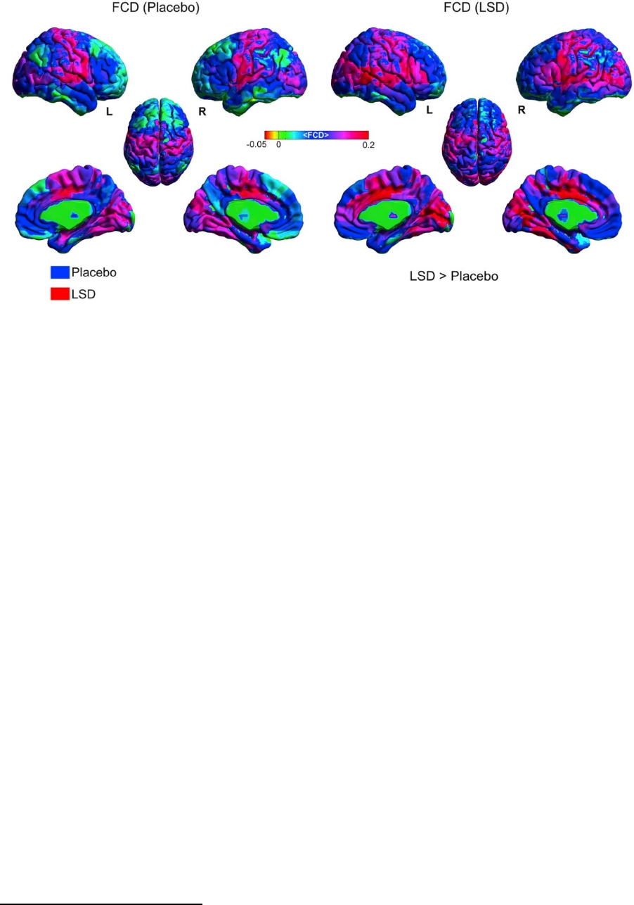
884
Figure 141. Average functional connectivity density Φ under LSD vs. control condition
(adapted from Tagliazucchi et al., 2016, p. 1044)
The results demonstrate for the first time that LSD increases global inter-module
connectivity while at the same time decreasing the integrity of individual modules. The
observed changes in activity significantly correlated with the anatomical distribution of
5-HT
2A
receptors. Interestingly, LSD enhanced the connectivity between normally
separated brain networks (as quantified by the widely used Φ connectivity index
279
).
This result is especially relevant for researchers who want to identify the neural
correlates of creativity because an enhanced communication between previously
disconnected neuronal network modules is assumed to be crucial for the generation of
novel percepts and ideas (e.g., D. W. Moore et al., 2009). The authors concluded that
LSD reorganizes the rich-club architecture of brain networks and that this restructuring
is accompanied by a shift of the boundaries between self and environment. That is, the
279
The rich-club coefficient Φ is a networks metric which quantifies the degree to which well-connected
nodes (beyond a certain richness metric) also connect to each other. Hence, the rich-club coefficient can
be regarded as a notation which quantifies a certain type of associativity.

885
ego-based dichotomy between self and other, subject and object, internal and external,
dissolves as a function of specific connectivity changes in the modular networks of the
brain
280
.
Taken together, Tagliazucchi et al. (2016) demonstrate that LSD induced ego-
dissolution is accompanied by significant changes in the neuronal rich-club architecture
and that ego-dissolution is accompanied by the downregulation of the default-mode
network (DMN). In the context of creativity research this finding is particularly
intriguing because the DMN is associated with habitual thought and behavior patterns
which are hypothesized to be negatively correlated with creativity and the generation of
novel ideas. That is, downregulation of the DMN by psychedelics and the
accompanying phenomenology of ego-dissolution are promising factors for the
understanding (and enhancement) of creativity
281
.
Based on these findings, we suggest a novel neuropsychopharmacological
mechanism for the enhancement of creativity which has, to our best knowledge, never
been proposed before. We would like to emphasize the importance of ego-dissolution
for the enhancement of creativity, that is, a reduction of the influence of the ego (DMN)
on perception and cognition enables the percipient to perceive reality from a new (more
unbiased) perspective. Based on the hypothesis that ego-dissolution provides a
“cognitive reset” which enables us to perceive and conceptualize reality from a more
280
Furthermore, the authors argue convincingly that the notion that LSD (and other psychedelics)
“expand” consciousness is quantitatively supported by their data. Specifically, they argue that the
neurophysiological changes associated with psychedelic states contrast with states of diminished
consciousness (e.g., deep sleep or general anesthesia). The obtained results are congruent with the idea
that psychedelic and unconscious states can be conceptualized as polar-opposites on a continuous
spectrum of conscious states. Furthermore, the authors suggest that the level of consciousness is
quantitatively determined by the level of neuronal entropy (in accord with the entropic brain hypothesis
formulated by Carhart-Harris et al., 2014). It has been suggested that Aldous Huxley “reduction valve”
hypothesis appears to be relevant in this context.
281
Recent evidence focusing on changes in the coupling of electrophysiological brain oscillations by
means of transfer entropy suggests that serotonergic psychedelics temporarily change information transfer
(via an increase of entropy?) within neural hierarchies by decreasing frontal of top-down control, thereby
releasing posterior bottom-up information transfer from inhibition (Francesc Alonso et al., 2015).

886
unconstrained non-dualistic perspective, we argue that 5-MeO-DMT is an especially
intriguing molecule because its effects are much more pronounced than those of
psilocybin or LSD. The “reset theory” is a first attempt to conjecture a causal
mechanism which could explain why ego dissolution associated with the hypothesized
increase in creativity. See things with new eyes (entropy) with reduced influence of
perceptual schemata an a reduced top-down influence (i.e., preconception vs.
apperception). In sum, we argue that (e.g., psilocybin, DMT, 5-MeO-DMT) are
catalysts for though, imagination, understanding, and epiphany.
Ego-dissolution
Empirical data indicates that ego-dissolution is a unique property of certain
classes of psychedelic substances (Nour, Evans, Nutt, & Carhart-Harris, 2016b). In a
web-based study utilizing the Ego-Dissolution Inventory (EDI) several substances were
compared and the results showed that only psychedelics induced a compromised sense
of self. In the same study, participants also responded to a subset of items from the
Mystical Experiences Questionnaire (MEQ) with a significant factor loading on
“mystical experience” a defining feature of which is “unitive” (i.e., non-dual)
experience, as has already been pointed out by William James more than a century ago
(James, 1985/1902). Again, the results indicated that higher MEQ-scores were
associated with psychedelic substances but not with other psychoactive substance like
alcohol or cocaine.
5-MeO-DMT: An endogenous catalyst for creativity?
5-MeO-DMT (5-Methoxy-N,N-dimethyltryptamine) is a relatively unknown
member of a group of naturally-occurring psychoactive indolealkylamines. It is an
analog of tryptophan and endogenous to human physiology (Shen, Jiang, Winter, & Yu,
887
2010). Its extremely powerful acute effects are pharmacokinetically short-lived. As
many other tryptamine psychedelics, it acts as a nonselective 5-HT agonist
and causes a
broad spectrum of highly interesting psychological, effects. It displays a high binding
affinity for the 5-HT
1A
and 5-HT
2
and subtypes (Krebs-Thomson, Ruiz, Masten, Buell,
& Geyer, 2006) but other mechanism of actions appear to be involved in its
psychoactivity (e.g., inhibition of enzymatic monoamine oxidase activity; but see
Nagai, Nonaka, & Satoh Hisashi Kamimura, 2007). 5-MeO-DMT is widespread in the
plant kingdom and has been used by shamans for millennia (Torres et al., 1991).
While its structural relative Psilocybin is has only been found in fungi, 5-MeO-
DMT is present in various plants, for instance Virola theiodora (Agurell et al., 1969), a
tree species belonging to the Myristicaceae (nutmeg) family. In additions to its
relatively widespread phytochemical distribution, it is present in high concentrations in
the venom of Incilius alvarius (known as the Sonoran Desert toad), an Amphibia which
produces significant amounts of 5-Meo-DMT in its numerous parotoid glands as a
defensive chemical mechanism against predators (Erspamer, Vitali, Roseghini, & Cei,
1965; Hutchinson & Savitzky, 2004). The salience of toad symbolism in Mesoamerican
art and mythology is well documented by anthropologists and toad effigies (with
oftentimes accentuated glands) are prominent in the historical remains of the Mayan and
Aztec cultures (Davis & Weil, 1992). Moreover, 5-MeO-DMT can sometimes be found
in certain variations of Ayahuasca (a drinkable plant-based concoction, which is utilized
by indigenous tribes in the Amazonian rainforest for divinatory and healing purposes),
for instance, when the leaves of the plant “chaliponga” (Diplopterys cabrerana) are
added to the concoction (J. C. Callaway et al., 2006; Rätsch, 1998). 5-MeO-DMT has
been utilized for spiritual purposes as a religious sacrament in the rituals of the USA
based Christian “Church of the Tree of Life” (Gottlieb, 1994). Modern artworks

888
inspired by 5-MeO-DMT experiences are oftentimes geometrically complex and
reminiscent of multidimensional fractal-like mathematical structures. Despite its
longstanding usage in the course of human evolution
282
, systematic research is hitherto
very limited and science does not know much about the psychological effects of 5-
MeO-DMT. It has been convincingly argued that it is of is of “potential interest for
schizophrenia research owing to its hallucinogenic properties” and that research on 5-
MeO-DMT can “help to understand the neurobiological basis of hallucinations” (Riga,
Soria, Tudela, Artigas, & Celada, 2014)
283
even though visual hallucinations are much
less commonly reported compared to its structural analog N,N-Dimethyltryptamine
(DMT) which induced the most spectacular vivid visual perception possibly imaginable
(Strassman, 2001).
5-MeO-DMT exerts extremely profound effects on the self-concept (ego). Here,
the term ego is not used as defined in the classical Freudian tripartide model (Freud,
1923), but it refers to the concept of identity i.e., who we think we are as human beings.
Thus, the usage of the term ego is more closely aligned with the ancient Sanskrit term
“Ahaṃkāra” as defined in Vedic philosophy (cf. Cartesian positional identity; Comfort,
1979). In this theoretical/phenomenological framework, the ego can be conceptualized
as a filter or a lens which converts experiences. Pure awareness, on the other hand, lies
beyond the ego construct and is “that which perceives”. While the ego identifies with
282
The long history of human usage of this naturally occurring compound in various cultures suggests that
it does not convey a significant disadvantage in terms of evolutionary fitness i.e., natural selection (cf.
Martin & Nichols, 2017). Profit-oriented pharmaceutical companies, on the other hand, actively market
patented synthetic designer drugs which do not have any evolutionary track record and might cause all
kinds of unforeseen neurological, genetic, and epigenetic problems in the long run (cf. Y. Kim et al.,
2009), for instance, the widespread prescription of methylphenidate (e.g., Ritalin) in preschool children
(Keane, 2008), based on questionable DSM-5 nosology (Phillips et al., 2012b, 2012c, 2012d, 2012a). In
contrast to patentded pychopharmcological agents, there is no revenue model for psychedelics in the
classical sense.
283
An animal neuroimaging study conducted by Riga et al. (2014) showed that 5-MeO-DMT decreased
BOLD responses in the striate cortex (V1) and the medial prefrontal cortex (mPFC).

889
the content of sense experience, awareness itself does not (Sivananda, 1972). Awareness
itself has no associated identity. It is a detached witness of experience
284
.
5-MeO-DMT can occasion extremely profound non-dual experiences and it is
much more potent than its structural relatives (e.g., N,N-Dimethyltryptamine),
psychologically and quantitatively in terms of dosage. It has been described as a
prototypical entheogen (Metzner, 2015).
Given its phenomenological profundity and its unparalleled efficiency to
dissolve ego structures we propose that 5-MeO-DMT should be systematically
investigated in order to elucidate the postulated connection between non-dual (ego-less)
states of consciousness and the stipulated associated enhancement in creativity. The
main idea is that ego-dissolution is associated with a breakdown of linguistic structures
(hence the ineffability of its phenomenology). According to the Saphir-Whorf
hypothesis of linguistic relativism, language structures cognition and perception in
significant ways. Ergo, we hypothesize that a release from the strong aprioristic
influences of linguistic processes enables a more unrestrained style of cognition and
perception. We argue that the collapse of the “subject versus object” dichotomy into a
non-dual experience has enormous potential for complex cognitive restructuring. “Ego
death” (ego-dissolution) is emotionally and cognitively extremely challenging which
resonates with the “hardship model of creativity” (Forgeard, 2013). The experiences
induced by 5-MeO-DMT are tremendously radical
285
and therefore capable to disperse
284
Note that this statement is not an objective empirically validated ontological fact. It is based on
qualitative phenomenological experiences often induced by ego-dissolution (e.g., caused by meditation,
introspection, psychedelics, spontaneous epiphany, etc.). Ego-less pure awareness plays a central role in
many ancient philosophical schools of thought (Mahayana and Zen Buddhism, Advaita Vedanta, Taoism,
Sufism, ect. pp.).
285
It has been argued elsewhere that “increased creativity may … constitute a manifestation of
posttraumatic growth, defined as retrospective perceptions of positive psychological changes that take
place following experiences of highly challenging life circumstances” (Forgeard, 2013, p. 245).

890
deeply engrained cognitive/perceptual schemata
286
, thereby enabling a more
unrestricted style of cognition
287
. Specifically, we argue that it facilitates a less self-
centered and hence more unbiased style of cognition. This hypothesis is empirically
testable hypothesis which is experimentally falsifiable in the Popperian sense. Various
cognitive testing procedures
288
could be utilized to investigate this claim. For instance,
we predict a reduction of various cognitive and perceptual biases (Kahneman &
Tversky, 1974) after 5-MeO-DMT administration due to enhancements in “openness to
experience” (cf. MacLean et al., 2011; Silvia et al., 2009) and alterations in “epistemic
style” (Eigenberger et al., 2007). Various dual-process models of cognition (Jonathan St
B T Evans, 2008) might prove to be relevant in this context. Limitations of space do not
allow us to discuss the multifarious details of this empirical agenda. Hence, we leave
the reader with the adumbration that 5-MeO-DMT might be a very fruitful
neurochemical research tool for future neuroscientific/psychological studies
289
,
specifically in the context of ego-dissolution and the catalysis of creativity. Anecdotal
evidence suggests that creativity originates from states of mind in which the ego-
function is reduced, and mental contents are allowed to “flow” in an uninhibited
manner. Both artists and athletes understand that thinking can interfere with creative
286
Interestingly, preliminary evidence suggests that it is effective in the treatment of addiction,
depression, and obsessive-compulsive disorders (Bogenschutz et al., 2015; Carhart-Harris, Bolstridge, et
al., 2016). This is congruent with the formulated idea that 5-MeO-DMT has the potential to change
persistent habitual modes of thought.
287
This idea could be empirically tested, for instance, by utilizing a semantic priming paradigm in order
to investigate spread of activation (as proxy for verbal creativity). Exemplary studies have been
conducted with the dopamine precursor L-Dopa by, for example, Kischka et al. (1996) in order to
elucidate the role of dopaminergic neurotransmission in verbal creativity. Anecdotal evidence suggest that
serotonergic psychedelics can enhance verbal creativity significantly (longitudinally). In the acute phase,
many psychedelics interfere strongly with the linguistic system (a breakdown of semantic and syntactic
facilities is oftentimes reported). Interesting, glossolalia is reported in a few cases.
288
It should be noted that psychedelic might cause serious psychological harm to certain populations with
psychopathological dispositions (e.g., specific 5-HT receptor polymorphism). Ergo, careful a priori
screening is crucial for ethically responsible research.
289
5-MeO-DMT has a very fast onset and a short duration (< 1 hour as opposed to opposed to the long
duration of LSD and Psilocybin (several hours) which makes it particularly attractive from a
methodological point of view.

891
performance. This theory is congruent with various dual-system accounts of cognition
(Eigenberger et al., 2007; Jonathan St B T Evans, 2008; Kahneman, 2003), i.e., system
1 processes are less constrained by system 2 processes leading to a more “unconstrained
style of cognition”).
The logical which undergirds our theorizing can be formalized as a syllogistic deductive
argument (modus ponens):
1
st
premise:
2
nd
premise:
Conclusion:
The phenomenological experiences associated with ego-dissolution
enhance creativity.
5-MeO-DMT catalyses ego-dissolution.
Ergo, 5-MeO-DMT enhances creativity (via the proxy of ego-
dissolution).
Based on this background, we postulate the following more specific directional
hypotheses:
Hypothesis 1: The intensity of ego-dissolution experienced by participants predicts the
longitudinally measured significance of the life-event in a non-linear dose-dependent
manner (Griffiths, Richards, Johnson, McCann, & Jesse, 2008).
Hypothesis 2: Self-reported ego-dissolution predicts subsequent enhancements in
creativity, as quantified by various test batteries (e.g., J. C. Kaufman, 2012). This effect
is mediated by the profundity of the experience, e.g., how challenging the experience
was, intensity of the “peak experience” , personal meaningfulness of the experience, etc.
(Barrett, Bradstreet, Leoutsakos, Johnson, & Griffiths, 2016; Forgeard, 2013; Griffiths
et al., 2006; Majić, Schmidt, & Gallinat, 2015).
Hypothesis 3: The intensity of 5-MeO-DMT induced ego-dissolution predicts
consequent increases in aesthetic perception/apperception, biophilia, and feelings of
fundamental existential interconnectedness (viz., “nonduality”).

892
We argue that the hypothesized effects are objectively quantifiable (i.e., measurable)
and repeatable in rigorously controlled experimental settings.
Brains in chains: Neurodiversity and cognitive liberty
The UK is the first country in human history which generically bans all
psychoactive substances, i.e., an omnibus prohibition of all mind-altering chemicals,
irrespective of their well-documented historical use and their safety profile, for
example, as objectively quantified by the conventional LD
50
and TD
50
toxicity indices.
For instance, psilocybin exhibits remarkably low toxicity. The LD
50
in humans remains
unknown, given the lack of any intentional or accidental poisoning death data. The
therapeutic window (or pharmaceutical window) is extremely safe and the maximum
tolerated dose (MTD) is very high, i.e., the therapeutic index is very high.
290
A common
metric in comparative risk assessment is the margin of exposure (MOE), defined as the
ratio between the toxicological threshold (defined as the benchmark dose) and the
estimated average human intake (Lachenmeier & Rehm, 2015). Both, MTD and MOE
indicate a very benign safety profile for psilocybin, especially compared to neurotoxic
agents like alcohol which has a very low MOE (Lachenmeier & Rehm, 2015) and has
been associated with numerous detrimental neurocognitive (Weitemier & Ryabinin,
2003), genetic, and epigenetic effects (Y. Chen, Ozturk, & Zhou, 2013). Despite these
factoids, psilocybin is classified as a class A substance in the UK
291
. This Regulation is
290
Alcohol, which is legal and indeed systematically promoted by the alcohol industry, has a very unsafe
LD
50
profile and is proven to be neurotoxic (R. Da Lee et al., 2005; Jacobus & Tapert, 2013). Recent
longitudinal research has shown that even moderate alcohol consumption has detrimental effects on
various neuroanatomical structures (e.g., hippocampal atrophy). Psilocybin, on the other hand, has been
shown to induce neurogenesis in the hippocampus in animal studies (Catlow et al., 2013).
291
In the USA it is also in the highest category (Schedule 1) even though none of the classification
criteria apply to psilocybin. For instance, to be classified as a Schedule 1 substance, a given chemical
must have “high potential for abuse” and “no accepted medical use”. Both criteria do not apply to
psilocybin which has been successfully used in medical contexts to treat addiction (Bogenschutz &
Johnson, 2016) and depression (Griffiths et al., 2016), inter alia. Ergo, the classification is clearly not
rationally justifiable, but see https://www.dea.gov/druginfo/ds.shtml

893
a lex specialis, which introduces an additional serious burden for researchers interested
in non-ordinary states of consciousness. Regrettably, scientific research on psychedelics
is currently legally highly restricted due to the irrational Class A status of psychedelic
substances as defined in the “Psychoactive Substances Act
292
” (PSA) which reached
Royal Assent in January 2016. The PSA generically prohibits all mind-altering
substances besides the most harmful and addictive ones which are of commercial
significance (e.g., alcohol and tobacco; but see Nutt, King, & Phillips, 2010) and it
classifies relatively harmless substances like psilocybin on par the most harmful and
detrimental substances like heroin, cocaine, and alcohol. This classification is based on
the assumption that psilocybin has no medicinal value which is clearly not the case (but
see Bogenschutz & Johnson, 2016). The widespread psychological propaganda (E. L.
Bernays, 1928, 1936; Mullen, 2010) against psychedelics (linking psychedelic use to
psychopathology and suicide) which was initiated by Nixon’s “war on drugs”
campaign, has now been evidently debunked (Johansen & Krebs, 2015), even though
the public mind is still under its influence. Well informed legal scholars interpret the
PSA as an explicit violation of the right to mental self-determination (i.e., cognitive
liberty; Walsh, 2016) – particularly in the context of Article 9 of the European
Convention on Human Rights which should protect the right to freedom of thought.
Freedom of thought is an axiomatic precursor to various other liberties like the freedom
of speech. Or as United States Supreme Court formulated it: “freedom of thought … is
the matrix, the indispensable condition, of nearly every other form of freedom”
(“PALKO v. STATE OF CONNECTICUT,” n.d.). Furthermore, it is self-evident that
cognitive liberty is a prerequisite for creativity. It can be convincingly argued that the
PSA reduces neurodiversity - it homogenizes cognitive/neuronal processes and restricts
292
For more information see http://www.legislation.gov.uk/ukpga/2016/2/contents/enacted
894
memetic and, ergo, cultural memetic evolution (in analogy with the importance of
genetic diversity in the context of biological evolution). Humanity does not know which
ideas will be important in the future. Memetic variability is as important to humanity as
is genetic variability due to the unpredictability of future environments.
Summa summarum, the PSA is factually not evidence-based and presents a serious legal
impediment to scientific research, neurodiversity, and creativity (see also Boire, 2000).
Conclusion
We would like to close with some general remarks. So far, contemporary science has
largely neglected the extraordinary experiences catalyzed by psychedelics. In his
classic book entitled “The structure of scientific revolutions”, Thomas Kuhn pointed out
that it is general phenomenon that paradigm challenging anomalies “that subvert the
existing tradition of scientific practice” (T. Kuhn, 1970, p. 6) are neglected as long as
possible. Research on psychedelics might force us the rethink our most fundamental
beliefs about the way we conceive reality and practice science (e.g., the stipulated
dichotomy between observer and observed; physicalism/the brain produces
consciousness, etc.) and is therefore implicitly perceived as a threat to the widely
adopted “quasi-Newtonian” status quo which, in reality, has already been thoroughly
revised by quantum physics (e.g., the implications of violations of Bell inequalities for
“local realism”, Gröblacher et al., 2007; Handsteiner et al., 2017). A detached dualistic
“objective” science is no longer possible due to the firmly established holistic nature of
quantum entanglement (Horodecki, Horodecki, Horodecki, & Horodecki, 2009). If
science wants to live up to its ideal to capture reality in its entirety without leaving any
residue, then it needs to integrate psychedelics into its modelling efforts – especially
given the fact that many psychoactive alkaloids are endogenous components of human
neurochemistry and ergo arguably of evolutionary relevance. Any model which
895
incorporates only a specific (selected) subset of the available quantitative and
qualitative data is necessarily at best incomplete (and in the worst case scenario
prejudiced, dogmatic, and systematically biased). We are confident that a mature
science will sooner or later investigate these naturally occurring compounds in the
context of human psychology. It’s just a matter of time…
We would like to close with an apposite quote from William James (who experimented
with Nitrous Oxide and the psychedelic Mescaline himself). He articulated in his classic
“Essays in Radical Empiricism”:
"To be radical, an empiricist must neither admit into his constructions any element that
is not directly experienced, nor exclude from them any element that is directly
experienced" (James, 1912/1976, p.42).
896
References
Agurell, S., Holmstedt, B., Lindgren, J.-E., Schultes, R. E., Lindberg, A. A., Jansen, G.,
… Samuelsson, B. (1969). Alkaloids in Certain Species of Virola and Other South
American Plants of Ethnopharmacologic Interest. Acta Chemica Scandinavica, 23, 903–
916. https://doi.org/10.3891/acta.chem.scand.23-0903
Amin, A. H., Crawford, T. B. B., & Gaddum, J. H. (1954). The distribution of substance
P and 5-hydroxytryptamine in the central nervous system of the dog. Journal of
Physiology, 596–618.
Baddeley, A. (1992). Working Memory. Science, 255(5044), 556–559.
https://doi.org/10.1126/science.1736359
Barrett, F. S., Bradstreet, M. P., Leoutsakos, J.-M. S., Johnson, M. W., & Griffiths, R.
R. (2016). The Challenging Experience Questionnaire: Characterization of challenging
experiences with psilocybin mushrooms. Journal of Psychopharmacology, 30(12),
1279–1295. https://doi.org/10.1177/0269881116678781
Bernays, E. L. (1928). Propaganda. Horace Liveright.
Bernays, E. L. (1936). Freedom of Propaganda. Vital Speeches of the Day, 2(24), 744–
746.
Blutner, R., Pothos, E. M., & Bruza, P. (2013). A quantum probability perspective on
borderline vagueness. Topics in Cognitive Science, 5(4), 711–736.
https://doi.org/10.1111/tops.12041
Bogenschutz, M. P., Forcehimes, A. A., Pommy, J. A., Wilcox, C. E., Barbosa, P. C. R.,
& Strassman, R. J. (2015). Psilocybin-assisted treatment for alcohol dependence : A
897
proof-of-concept study. Journal of Psychopharmacology, 29(3), 289–299.
https://doi.org/10.1177/0269881114565144
Bogenschutz, M. P., & Johnson, M. W. (2016). Classic hallucinogens in the treatment
of addictions. Progress in Neuro-Psychopharmacology and Biological Psychiatry, 64,
250–258. https://doi.org/10.1016/j.pnpbp.2015.03.002
Boire, R. (2000). On Cognitive Liberty. Journal of Cognitive Liberties, 1(1), 1–26.
Bolstridge, M. (2013). The Psychedelic Renaissance: Reassessing the Role of
Psychedelic Drugs in 21st Century Psychiatry and Society. The British Journal of
Psychiatry, 202(3), 239–239. https://doi.org/10.1192/bjp.bp.112.122481
Callaway, J. C., Grob, C. S., McKenna, D. J., Nichols, D. E., Shulgins, A., & Tupper,
K. W. (2006). A Demand for Clarity Regarding a Case Report on the Ingestion of 5-
Methoxy-N, N-Dimethyltryptamine (5-MeO-DMT) in an Ayahuasca Preparation.
Journal of Analytical Toxicology, 30(6), 406–407. https://doi.org/10.1093/jat/30.6.406
Carhart-Harris, R. L., Bolstridge, M., Rucker, J., Day, C. M. J., Erritzoe, D., Kaelen,
M., … Nutt, D. J. (2016). Psilocybin with pyschological support for treatment-resistant
depression: an open-label feasibility study. The Lancet Psychiatry, 3(7), 619–627.
https://doi.org/10.1016/S2215-0366(16)30065-7
Carhart-Harris, R. L., Leech, R., Hellyer, P. J., Shanahan, M., Feilding, A.,
Tagliazucchi, E., … Nutt, D. (2014). The entropic brain: a theory of conscious states
informed by neuroimaging research with psychedelic drugs. Frontiers in Human
Neuroscience, 8(February), 20. https://doi.org/10.3389/fnhum.2014.00020
Carhart-Harris, R. L., & Nutt, D. J. (2017). Serotonin and brain function: A tale of two
receptors. Journal of Psychopharmacology. https://doi.org/10.1177/0269881117725915
898
Catlow, B. J., Song, S., Paredes, D. A., Kirstein, C. L., & Sanchez-Ramos, J. (2013).
Effects of psilocybin on hippocampal neurogenesis and extinction of trace fear
conditioning. Experimental Brain Research, 228(4), 481–491.
https://doi.org/10.1007/s00221-013-3579-0
Chen, Y., Ozturk, N. C., & Zhou, F. C. (2013). DNA Methylation Program in
Developing Hippocampus and Its Alteration by Alcohol. PLoS ONE, 8(3).
https://doi.org/10.1371/journal.pone.0060503
Comfort, A. (1979). The Cartesian observer revisited: ontological implications of the
homuncular illusion. Journal of Social and Biological Systems, 2(3), 211–223.
https://doi.org/10.1016/0140-1750(79)90028-9
Da Lee, R., Mi An, S., Sun Kim, S., Seek Rhee, G., Jun Kwack, S., Hyun Seok, J., …
Lea Park, K. (2005). Neurotoxic Effects of Alcohol and Acetaldehyde During
Embryonic Development. Journal of Toxicology and Environmental Health, Part A,
68(23–24), 2147–2162. https://doi.org/10.1080/15287390500177255
Davis, W., & Weil, A. T. (1992). Identity of a New World Psychoactive Toad. Ancient
Mesoamerica, 3(1), 51–59. https://doi.org/10.1017/S0956536100002297
Davis, J. V. (2011). Ecopsychology, transpersonal psychology, and nonduality.
International Journal of Transpersonal Studies.
https://doi.org/10.1002/9781118591277.ch33
Della Sala, S., Gray, C., Spinnler, H., & Trivelli, C. (1998). Frontal lobe functioning in
man: The riddle revisited. Archives of Clinical Neuropsychology, 13(8), 663–682.
https://doi.org/10.1016/S0887-6177(97)00093-0
899
DeYoung, C. G., Peterson, J. B., & Higgins, D. M. (2005). Sources of
Openness/Intellect: Cognitive and neuropsychological correlates of the fifth factor of
personality. Journal of Personality. https://doi.org/10.1111/j.1467-6494.2005.00330.x
Eigenberger, M. E., Critchley, C., & Sealander, K. A. (2007). Individual differences in
epistemic style: A dual-process perspective. Journal of Research in Personality, 41(1),
3–24. https://doi.org/10.1016/j.jrp.2006.01.003
Erspamer, V., Vitali, T., Roseghini, M., & Cei, J. M. (1965). 5-Methoxy- and 5-
hydroxy-indolealkylamines in the skin of Bufo alvarius. Experientia, 21(9), 504.
https://doi.org/10.1007/BF02138956
Evans, J. S. B. T. (2008). Dual-processing accounts of reasoning, judgment, and social
cognition. Annual Review of Psychology, 59, 255–278.
https://doi.org/10.1146/annurev.psych.59.103006.093629
Feist, G. J. (1998). A Meta-Analysis of Personality in Scientific and Artistic Creativity.
Personality and Social Psychology Review, 2(4), 290–309.
https://doi.org/10.1207/s15327957pspr0204_5
Flexner, A. (n.d.). THE USEFULNESS OF USELESS KNOWLEDGE. Retrieved from
https://library.ias.edu/files/UsefulnessHarpers.pdf
Fontanilla, D., Johannessen, M., Hajipour, A. R., Cozzi, N. V., Jackson, M. B., &
Ruoho, A. E. (2009). The hallucinogen N,N-dimethyltryptamine (DMT) is an
endogenous sigma-1 receptor regulator. Science, 323(5916), 934–937.
https://doi.org/10.1126/science.1166127
900
Forgeard, M. J. C. (2013). Perceiving benefits after adversity: The relationship between
self-reported posttraumatic growth and creativity. Psychology of Aesthetics, Creativity,
and the Arts, 7(3), 245–264. https://doi.org/10.1037/a0031223
Francesc Alonso, J., Romero, S., Angel Mañanas, M., & Riba, J. (2015). Serotonergic
psychedelics temporarily modify information transfer in humans. International Journal
of Neuropsychopharmacology, 18(8), 1–9. https://doi.org/10.1093/ijnp/pyv039
Freud, S. (1923). The Ego and the Id. The Standard Edition of the Complete
Psychological Works of Sigmund Freud, Volume XIX (1923-1925): The Ego and the Id
and Other Works, 19–27. https://doi.org/10.1097/00000441-196111000-00027
Freud, S. (1939). Die Traumdeutung. Leipzig und Wien: Franz Deuticke.
Gaddum, J. H., & Hameed, K. A. (1954). Drugs which antagonize 5-
hydroxytryptamine. British Journal of Pharmacology, 240–248.
Gottlieb, A. (1994). Legal highs : a concise encyclopedia of legal herbs &
chemicals with psychoactive properties. Ronin Pub.
Grey, A. (2001). Transfigurations. Rochester, VT: Inner Traditions.
Griffiths, R. R., Johnson, M. W., Carducci, M. A., Umbricht, A., Richards, W. A.,
Richards, B. D., … Klinedinst, M. A. (2016). Psilocybin produces substantial and
sustained decreases in depression and anxiety in patients with life-threatening cancer: A
randomized double-blind trial. Journal of Psychopharmacology, 30(12), 1181–1197.
https://doi.org/10.1177/0269881116675513
Griffiths, R. R., Richards, W. A., McCann, U., & Jesse, R. (2006). Psilocybin can
occasion mystical-type experiences having substantial and sustained personal meaning
901
and spiritual significance. Psychopharmacology, 187(3), 268–283.
https://doi.org/10.1007/s00213-006-0457-5
Griffiths, R. R., Richards, W., Johnson, M., McCann, U., & Jesse, R. (2008). Mystical-
type experiences occasioned by psilocybin mediate the attribution of personal meaning
and spiritual significance 14 months later. Journal of Psychopharmacology (Oxford,
England), 22(6), 621–32. https://doi.org/10.1177/0269881108094300
Gröblacher, S., Paterek, T., Kaltenbaek, R., Brukner, Č., Zukowski, M., Aspelmeyer,
M., & Zeilinger, A. (2007). An experimental test of non-local realism. Nature,
446(7138), 871–875. https://doi.org/10.1038/nature05677
Handsteiner, J., Friedman, A. S., Rauch, D., Gallicchio, J., Liu, B., Hosp, H., …
Zeilinger, A. (2017). Cosmic Bell Test: Measurement Settings from Milky Way Stars.
Physical Review Letters, 118(6). https://doi.org/10.1103/PhysRevLett.118.060401
Harman, W. W., McKim, R. H., Mogar, R. E., Fadiman, J., & Stolaroff, M. J. (1966).
Psychedelic agents in creative problem-solving: a pilot study. Psychological Reports,
19(1), 211–227. https://doi.org/10.2466/pr0.1966.19.1.211
Hofmann, A., Frey, A., Ott, H., Petrzilka, T., & Troxler, F. (1958). Elucidation of the
structure and the synthesis of psilocybin. Experientia, 14(11), 397–399.
https://doi.org/10.1007/BF02160424
Hofmann, A., Heim, R., Brack, A., Kobel, H., Frey, H., Ott, H., … Troxler, F. (1959).
Psilocybin und Psilocin, zwei psychotrope Wirkstoffe aus mexikanischen Rauschpilzen.
Helvetica Chimica Acta, 42, 1557–1572.
902
Horodecki, R., Horodecki, P., Horodecki, M., & Horodecki, K. (2009). Quantum
entanglement. Reviews of Modern Physics, 81(2), 865–942.
https://doi.org/10.1103/RevModPhys.81.865
Hutchinson, D. A., & Savitzky, A. H. (2004). Vasculature of the parotoid glands of four
species of toads (Bufonidae: Bufo). Journal of Morphology, 260(2), 247–254.
https://doi.org/10.1002/jmor.10219
Huxley, A. (1954). The Doors of Perception and Heaven and Hell. Harper & Brothers,
London.
Ivcevic, Z., & Brackett, M. A. (2015). Predicting Creativity: Interactive effects of
openness to experience and emotion regulation ability. Psychology of Aesthetics,
Creativity, and the Arts, 9(4), 480–487.
https://doi.org/http://dx.doi.org/10.1037/a0039826
Jacobus, J., & Tapert, S. F. (2013). Neurotoxic Effects of Alcohol in Adolescence.
Annual Review of Clinical Psychology, 9(1), 703–721. https://doi.org/10.1146/annurev-
clinpsy-050212-185610
James, W. (1976). Essays in radical empiricism. Harvard University Press.
James, W. (1985). The Varieties of Religious Experience: A Study in Human Nature.
London: Penguin Classics. (Originally published in 1902).
Johansen, P.-Ø., & Krebs, T. S. (2015). Psychedelics not linked to mental health
problems or suicidal behavior: A population study. Journal of Psychopharmacology,
29(3), 270–279. https://doi.org/10.1177/0269881114568039
903
Jung, C. G. (1969). Aion: Researches into the Phenomenology of the Self, Collected
Works of C. G. Jung (Volume 9). Princeton, N.J.: Princeton University Press.
Kahneman, D. (2003). Maps of bounded rationality: Psychology for behavioral
economics. American Economic Review. https://doi.org/10.1257/000282803322655392
Kahneman, D., & Tversky, A. (1974). Judgment under uncertainty: heuristics and
biases. Science, 185(4157), 1124–1131. https://doi.org/10.1126/science.185.4157.1124
Kandel, R. E. (2015). The Age of Insight: The Quest to Understand the Unconscious in
Art, Mind and Brain. The effects of brief mindfulness intervention on acute pain
experience: An examination of individual difference (Vol. 1).
https://doi.org/10.1017/CBO9781107415324.004
Kaufman, J. C. (2012). Counting the muses: Development of the Kaufman Domains of
Creativity Scale (K-DOCS). Psychology of Aesthetics, Creativity, and the Arts, 6(4),
298–308. https://doi.org/10.1037/a0029751
Kaufman, S. B., Quilty, L. C., Grazioplene, R. G., Hirsh, J. B., Gray, J. R., Peterson, J.
B., & Deyoung, C. G. (2016). Openness to Experience and Intellect Differentially
Predict Creative Achievement in the Arts and Sciences. Journal of Personality, 84(2),
248–258. https://doi.org/10.1111/jopy.12156
Keane, H. (2008). Pleasure and discipline in the uses of Ritalin. International Journal of
Drug Policy, 19(5), 401–409. https://doi.org/10.1016/j.drugpo.2007.08.002
Kekulé, A. (1866). Untersuchungen über aromatische Verbindungen. Annalen Der
Chemie Und Pharmacie, 137(2), 129–196. https://doi.org/10.1002/jlac.18661370202.
904
Kekulé, A. (1890). Benzolfest: Rede. Berichte Der Deutschen Chemischen Gesellschaft,
23(1), 1302–1311. https://doi.org/10.1002/cber.189002301204
Kerns, J. G., Cohen, J. D., MacDonald, A. W., Cho, R. Y., Stenger, V. A., & Carter, C.
S. (2004). Anterior Cingulate Conflict Monitoring and Adjustments in Control. Science,
303(5660), 1023–1026. https://doi.org/10.1126/science.1089910
Kim, Y., Teylan, M. A., Baron, M., Sands, A., Nairn, A. C., & Greengard, P. (2009).
Methylphenidate-induced dendritic spine formation and DeltaFosB expression in
nucleus accumbens. Proceedings of the National Academy of Sciences of the United
States of America, 106(8), 2915–20. https://doi.org/10.1073/pnas.0813179106
Kischka, U., Kammer, T. H., Maier, S., Weisbrod, M., Thimm, M., & Spitzer, M.
(1996). Dopaminergic modulation of semantic network activation. Neuropsychologia,
34(11), 1107–1113. https://doi.org/10.1016/0028-3932(96)00024-3
Kuhn, T. (1970). The Structure of Scientific Revolutions. University of Chicago Press,
University of Chicago.
Lachenmeier, D. W., & Rehm, J. (2015). Comparative risk assessment of alcohol,
tobacco, cannabis and other illicit drugs using the margin of exposure approach.
Scientific Reports, 5. https://doi.org/10.1038/srep08126
Lyons, T., & Carhart-Harris, R. L. (2018). Increased nature relatedness and decreased
authoritarian political views after psilocybin for treatment-resistant depression. Journal
of Psychopharmacology, 26988111774890. https://doi.org/10.1177/0269881117748902
MacLean, K. A., Johnson, M. W., & Griffiths, R. R. (2011). Mystical experiences
occasioned by the hallucinogen psilocybin lead to increases in the personality domain of
905
openness. Journal of Psychopharmacology, 25(11), 1453–1461.
https://doi.org/10.1177/0269881111420188
Madarasz, T. J., Diaz-Mataix, L., Akhand, O., Ycu, E. A., LeDoux, J. E., & Johansen, J.
P. (2016). Evaluation of ambiguous associations in the amygdala by learning the
structure of the environment. Nature Neuroscience, 19(7), 965–972.
https://doi.org/10.1038/nn.4308
Majić, T., Schmidt, T. T., & Gallinat, J. (2015). Peak experiences and the afterglow
phenomenon: When and how do therapeutic effects of hallucinogens depend on
psychedelic experiences? Journal of Psychopharmacology, 29(3), 241–253.
https://doi.org/10.1177/0269881114568040
Markoff, J. (2005). What the Dormouse Said: How the Sixties Counterculture Shaped
the Personal Computer Industry. New York: Viking.
Martin, D. A., & Nichols, C. D. (2017). The Effects of Hallucinogens on Gene
Expression. In Current topics in behavioral neurosciences.
https://doi.org/10.1007/7854_2017_479
Maslow, A. (1968). Toward a psychology of being. 2nd ed. Toward a psychology of
being. 2nd ed.
Maslow, A. (1972). The farther reaches of human nature. New York: Arkana.
Meneses, A. (1999). 5-HT system and cognition. Neuroscience and Biobehavioral
Reviews. https://doi.org/10.1016/S0149-7634(99)00067-6
Metzner, R. (2015). Allies for awakening : guidelines for productive and safe
experiences with entheogens. Berkeley, CA: Green Earth Foundation & Regent Press.
906
Moore, D. W., Bhadelia, R. A., Billings, R. L., Fulwiler, C., Heilman, K. M., Rood, K.
M. J., & Gansler, D. A. (2009). Hemispheric connectivity and the visual-spatial
divergent-thinking component of creativity. Brain and Cognition, 70(3), 267–272.
https://doi.org/10.1016/j.bandc.2009.02.011
Mullen, A. (2010). Twenty years on: the second-order prediction of the Herman--
Chomsky Propaganda Model. Media, Culture & Society, 32(4), 673–690.
https://doi.org/10.1177/0163443710367714
Mullis, K. (2000). Dancing naked in the mind field. New York: Vintage Books.
Retrieved from https://archive.org/details/DancingNakedInTheMindField-PDF
Nagai, F., Nonaka, R., & Satoh Hisashi Kamimura, K. (2007). The effects of non-
medically used psychoactive drugs on monoamine neurotransmission in rat brain.
European Journal of Pharmacology, 559(2–3), 132–137.
https://doi.org/10.1016/j.ejphar.2006.11.075
Nelson, T. (1975). Computer Lib/Dream Machines. South Bend: Nelson.
Nichols, D. E. (2004). Hallucinogens. Pharmacology and Therapeutics.
https://doi.org/10.1016/j.pharmthera.2003.11.002
Nichols, D. E. (2016). Psychedelics. Pharmacological Reviews, 68(2), 264–355.
https://doi.org/10.1124/pr.115.011478
Nour, M. M., Evans, L., Nutt, D., & Carhart-Harris, R. L. (2016a). Ego-Dissolution and
Psychedelics: Validation of the Ego-Dissolution Inventory (EDI). Frontiers in Human
Neuroscience, 10(June), 269. https://doi.org/10.3389/fnhum.2016.00269
907
Nour, M. M., Evans, L., Nutt, D., & Carhart-Harris, R. L. (2016b). Ego-Dissolution and
Psychedelics: Validation of the Ego-Dissolution Inventory (EDI). Frontiers in Human
Neuroscience, 10, 269. https://doi.org/10.3389/fnhum.2016.00269
Nutt, D. J., King, L. A., & Phillips, L. D. (2010). Drug harms in the UK: A multicriteria
decision analysis. The Lancet, 376(9752), 1558–1565. https://doi.org/10.1016/S0140-
6736(10)61462-6
PALKO v. STATE OF CONNECTICUT. (n.d.). Retrieved February 17, 2018, from
http://caselaw.findlaw.com/us-supreme-court/302/319.html
Phillips, J., Frances, A., Cerullo, M. A., Chardavoyne, J., Decker, H. S., First, M. B., …
Zachar, P. (2012a). The six most essential questions in psychiatric diagnosis: A
pluralogue. Part 4: General conclusion. Philosophy, Ethics, and Humanities in
Medicine. https://doi.org/10.1186/1747-5341-7-14
Phillips, J., Frances, A., Cerullo, M. A., Chardavoyne, J., Decker, H. S., First, M. B., …
Zachar, P. (2012b). The six most essential questions in psychiatric diagnosis: A
pluralogue part 1: Conceptual and definitional issues in psychiatric diagnosis.
Philosophy, Ethics, and Humanities in Medicine. https://doi.org/10.1186/1747-5341-7-3
Phillips, J., Frances, A., Cerullo, M. A., Chardavoyne, J., Decker, H. S., First, M. B., …
Zachar, P. (2012c). The six most essential questions in psychiatric diagnosis: A
pluralogue part 2: Issues of conservatism and pragmatism in psychiatric diagnosis.
Philosophy, Ethics, and Humanities in Medicine. https://doi.org/10.1186/1747-5341-7-8
Phillips, J., Frances, A., Cerullo, M. A., Chardavoyne, J., Decker, H. S., First, M. B., …
Zachar, P. (2012d). The six most essential questions in psychiatric diagnosis: A
908
pluralogue part 3: Issues of utility and alternative approaches in psychiatric diagnosis.
Philosophy, Ethics, and Humanities in Medicine. https://doi.org/10.1186/1747-5341-7-9
Puccio, G. J. (2017). From the Dawn of Humanity to the 21st Century: Creativity as an
Enduring Survival Skill. In Journal of Creative Behavior (Vol. 51, pp. 330–334).
https://doi.org/10.1002/jocb.203
Putnam, H. (1983). Vagueness and alternative logic. Erkenntnis, 19(1–3), 297–314.
https://doi.org/10.1007/BF00174788
Rätsch, C. (1998). Enzyklopädie der psychoaktiven Pflanzen : Botanik,
Ethnopharmakologie und Anwendung. Wissenschaftliche Verlagsgesellschaft.
Riga, M. S., Soria, G., Tudela, R., Artigas, F., & Celada, P. (2014). The natural
hallucinogen 5-MeO-DMT, component of Ayahuasca, disrupts cortical function in rats:
reversal by antipsychotic drugs. The International Journal of
Neuropsychopharmacology, 17(8), 1269–1282.
https://doi.org/10.1017/S1461145714000261
Roberts, T. B. (2006). Psychedelic horizons : Snow White, immune system, multistate
mind, enlarging education. Imprint Academic.
Rocke, A. J. (2015). It began with a daydream: the 150th anniversary of the Kekulé
benzene structure. Angewandte Chemie (International Ed. in English), 54(1), 46–50.
https://doi.org/10.1002/anie.201408034
Schoch, R. (1994). A Conversation with Kerry Mullis. California Monthly, 105(1), 20.
909
Sessa, B. (2008). Is it time to revisit the role of psychedelic drugs in enhancing human
creativity? Journal of Psychopharmacology (Oxford, England), 22(8), 821–827.
https://doi.org/10.1177/0269881108091597
Sessa, B. (2012). Shaping the renaissance of psychedelic research. The Lancet,
380(9838), 200–201. https://doi.org/10.1016/S0140-6736(12)60600-X
Sheldrake, R., McKenna, T. K., Abraham, R., & Abraham, R. (2001). Chaos, creativity,
and cosmic consciousness. Park Street Press.
Shen, H.-W., Jiang, X.-L., Winter, J. C., & Yu, A.-M. (2010). Psychedelic 5-methoxy-
N,N-dimethyltryptamine: metabolism, pharmacokinetics, drug interactions, and
pharmacological actions. Current Drug Metabolism, 11(8), 659–66.
https://doi.org/10.1016/j.biotechadv.2011.08.021.Secreted
Silvia, P. J., Nusbaum, E. C., Berg, C., Martin, C., & O’Connor, A. (2009). Openness to
experience, plasticity, and creativity: Exploring lower-order, high-order, and interactive
effects. Journal of Research in Personality, 43(6), 1087–1090.
https://doi.org/10.1016/j.jrp.2009.04.015
Sivananda, S. R. I. S. (1972). Bhagavad gita. World, 23–24.
https://doi.org/10.1093/obo/9780195399318-0010
Slattery, D. (2015). Xenolinguistics : psychedelics, language, and the evolution of
consciousness. Berkeley, California: North Atlantic Books.
Strassman, R. (2001). DMT: the spirit molecule. Rochester, VT, (March), 7821.
Retrieved from http://scroungehound.com/SellSheets/B0145_DMT.pdf
910
Tagliazucchi, E., Roseman, L., Kaelen, M., Orban, C., Muthukumaraswamy, S. D.,
Murphy, K., … Carhart-Harris, R. (2016). Increased Global Functional Connectivity
Correlates with LSD-Induced Ego Dissolution. Current Biology, 26(8), 1043–1050.
https://doi.org/10.1016/j.cub.2016.02.010
Tart, C. T. (1972). States of Consciousness and State-Specific Sciences. Science (New
York, N.Y.), 176(4040), 1203–1210. https://doi.org/10.1126/science.176.4040.1203
Tart, C. T. (2008). Altered states of consciousness and the spiritual traditions: The
proposal for the creation of state-specific sciences. In Handbook of Indian psychology.
(pp. 577–609). https://doi.org/10.1017/UPO9788175968448.032
Torres, C. M., Repke, D. B., Chan, K., Mckenna, D., Llagostera, A., & Schultes, R. E.
(1991). Snuff Powders from Pre-Hispanic San Pedro de Atacama: Chemical and
Contextual Analysis. Current Anthropology, 32(5), 640–649.
Vartanian, O. (2013). Fostering Creativity: Insights from Neuroscience. In J. Vartanian,
O., Bristol, A. & Kaufman (Ed.), Neuroscience of Creativity (pp. 257–271). Cambridge,
MA: MIT Press. https://doi.org/10.7551/mitpress/9780262019583.003.0012
Walsh, C. (2016). Psychedelics and cognitive liberty: Reimagining drug policy through
the prism of human rights. International Journal of Drug Policy, 29, 80–87.
https://doi.org/10.1016/j.drugpo.2015.12.025
Watts, R., Day, C., Krzanowski, J., Nutt, D., & Carhart-Harris, R. (2017). Patients’
Accounts of Increased “Connectedness” and “Acceptance” After Psilocybin for
Treatment-Resistant Depression. Journal of Humanistic Psychology, 57(5), 520–564.
https://doi.org/10.1177/0022167817709585
911
Weitemier, A. Z., & Ryabinin, A. E. (2003). Alcohol-induced memory impairment in
trace fear conditioning: A hippocampus-specific effect. Hippocampus.
https://doi.org/10.1002/hipo.10063
Whitehead, A. N., & Russell, B. (1910). Principia mathematica (1st ed.). Cambridge:
Cambridge University Press.
Xie, G., Keyhani, N. O., Bonner, C. A., & Jensen, R. A. (2003). Ancient Origin of the
Tryptophan Operon and the Dynamics of Evolutionary Change. Microbiology and
Molecular Biology Reviews, 67(3), 303–342. https://doi.org/10.1128/MMBR.67.3.303-
342.2003

912
Vitæ auctoris
Name: Christopher Benjamin Germann
Date of birth: 06.03.1981
Place of birth: Germany, Berlin
______________________________________________________________________
Educational background
2005: Gertrud-Bäumer Berufskolleg Duisburg, Germany.
Abitur
2005-2009: Free University of Amsterdam, Netherlands.
Scientiæ Baccalaureus (Bachelor of Science) in Psychology.
Supervisor: Dr. Karen Mortier
2009-2010: University of Plymouth, United Kingdom.
Magister Scientiæ (Master of Science) in Psychological Research Methods (with
distinction).
Supervisor: Prof. Simon Handley
913
Research experience
I started studying psychology at the Free University of Amsterdam. My bachelor studies
(supervised by Dr. Karen Mortier) were conducted within the theoretical framework of
embodied cognition. In our experiments, we utilized different mood induction
techniques in order to empirically investigate their influence on selective attention in a
series of computerized visual search tasks. Our theorizing was significantly influenced
by considerations regarding conceptual metaphor theory and the neuropsychological
valence model of lateralised hemispheric processing of emotion perception.
Subsequent to my bachelor studies, I successfully completed a M.Sc. in psychological
research methods at the University of Plymouth. During my master's project, I
collaborated with Prof. Simon Handley and the resulting dissertation focused primarily
on the role executive functions play in syllogistic vs. belief-based reasoning (i.e., syntax
vs. semantics in belief bias). Much of the motivation for our experimentation was
derived from prior work on ego-depletion and contemporary dual process theories of
cognition. Based on this background, I acquired substantial knowledge in cognitive
psychology, particularly in the domain of reasoning and decision making (e.g., in the
Kahneman and Tversky research tradition).
Technical skills
I am a web and UI designer and proficient with modern information technologies
(HTML, CSS, JavaScript, PHP, etc.). Shortly after finishing my masters in
psychological research methods I started a webdesign company in Germany.

914
Personal interests
I am intrinsically very interested in the 5-hydroxytryptamine system and its role in
perception and cognition (for instance, creativity, neuroplasticity and neurogenesis).
Furthermore, philosophy of science and mind capture my deepest curiosity.
Personally, I love to exchange ideas with scholars who adhere to different scientific
paradigms because interdisciplinary discourse offers great intellectual stimulation and
provides impetus for the development of novel unconventional ideas.
“Be less curious about people and more curious about ideas.” ~Marie Curie
Oral presentation on quantum probability in visual perception:
http://irrational-decisions.com/uop/
Further information online:
http://www.cognovo.eu/christopher-germann
Contact via email:
mail@christopher-germann.de

915
End of thesis
916
917

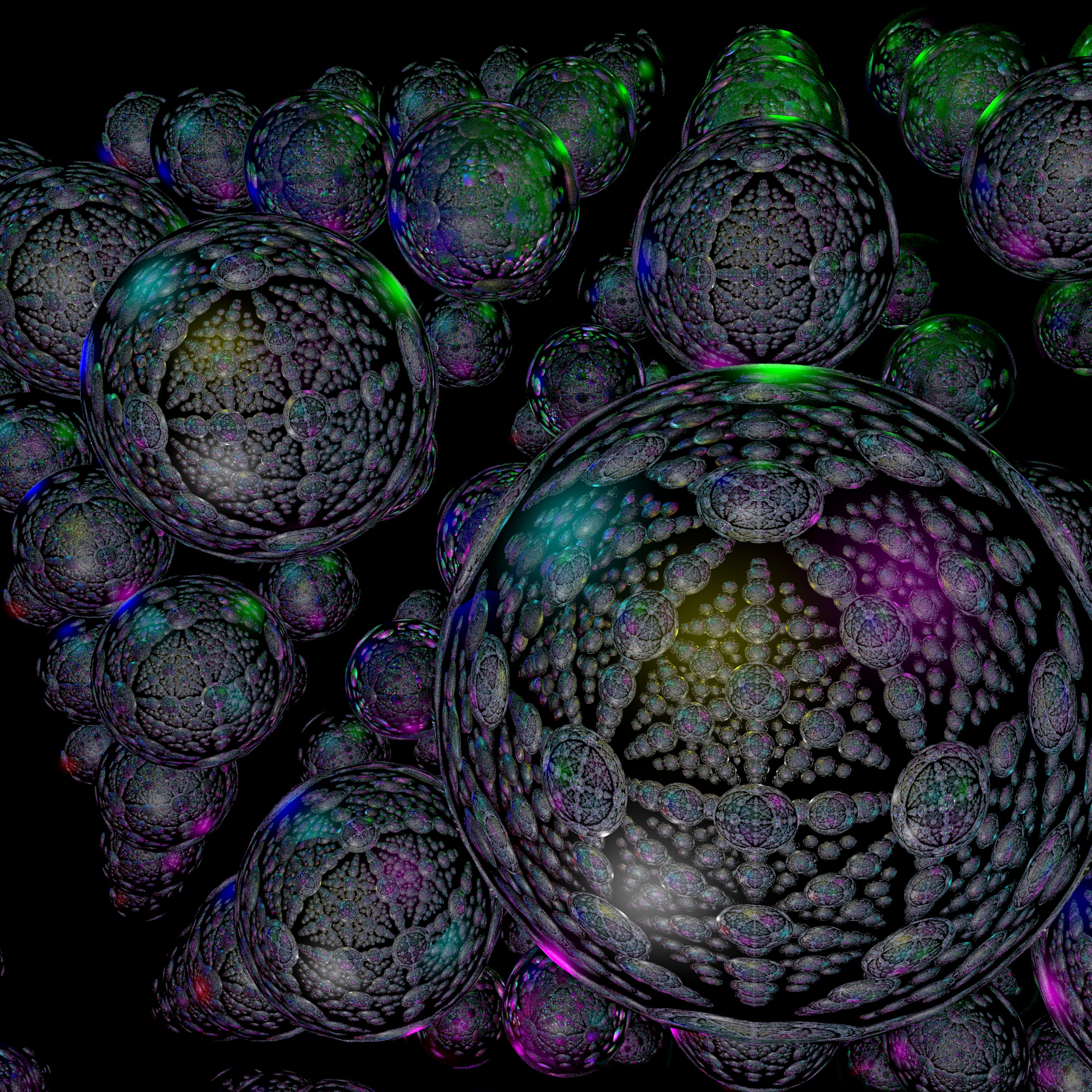