


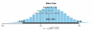
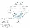
Figure 1. Visualisation of various Markov chain Monte Carlo convergence diagnostics for μ. MCMC convergence is a precondition which has to be satisfied in order to proceed with the Bayesian a posteriori parameter estimation.
Upper left panel: Trace plot: In order to examine the representativeness of the MCMC samples, we first visually examine the trajectory of the chains. The trace plot indicates convergence on θ, i.e., the trace plot appears to be stationary because its mean and variance are not changing as a function of time; ƒ(t).
Lower left panel: Shrink factor (Brooks-Gelman-Rubin statistic; Brooks & Gelman, 1997). Theoretically, the larger the number of iterations, the closer R should approximate 1 (as T → ∞, R → 1).
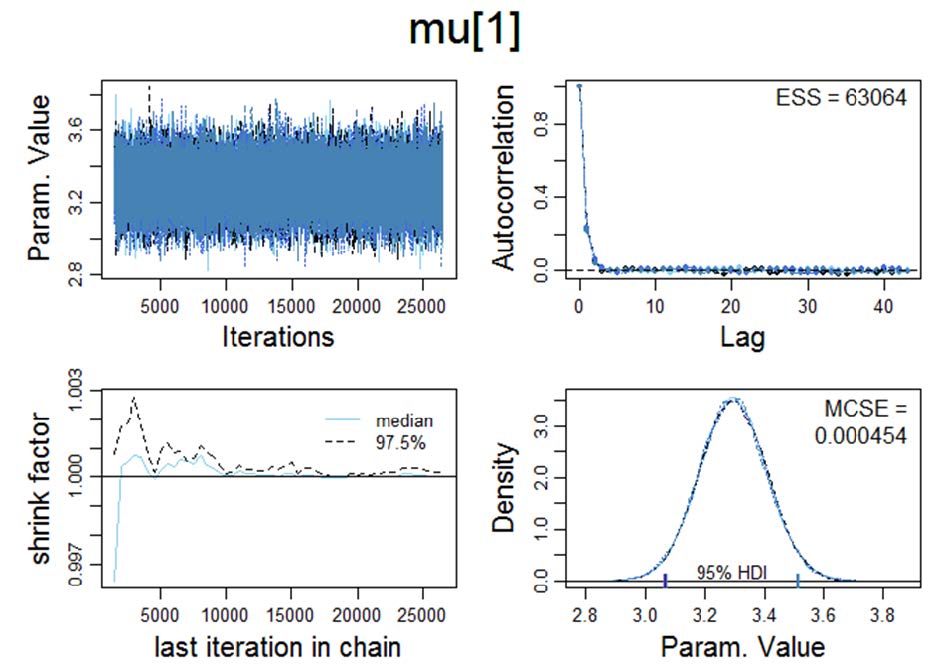
The MCMC between (B) and within-chain variance (W) is given by the following formula.*
*Footnote: In R this statistic can be computed with the coda package (which has numerous reverse depends, e.g., the Gibbs sampler JAGS/rjags). Coda provides functions for summarizing and plotting the output from Markov Chain Monte Carlo (MCMC) simulations, as well as diagnostic tests of convergence to the equilibrium distribution of the Markov chain.
CRAN: https://cran.r-project.org/web/packages/coda/coda.pdf
The "potential scale reduction factor" (shrink factor) is computed for each variable in x, together with the associated upper and lower confidence limits. Approximate convergence (equilibrium) is diagnosed when the upper limit ≈1.
gelman.diag(x, confidence = 0.95, transform=FALSE, autoburnin=TRUE, multivariate=TRUE)
gelman.plot(x, bin.width = 10, max.bins = 50,confidence = 0.95, transform = FALSE, autoburnin=TRUE, auto.layout = TRUE,ask, col, lty, xlab, ylab, type, ...)
The full code can be found on my website: http://r-code.ml
If you have any R-ode you would like to share with the world you can submit it via the HTML-form.
References
- Brooks, SP. and Gelman, A. (1997) General methods for monitoring convergence of iterative simulations. Journal of Computational and Graphical Statistics, 7, 434-455.
- Plummer, M. (2016). JAGS Version 4.3.0.http://mcmc-jags.sourceforge.net/
General remarks
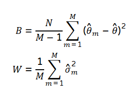
Based on my practical experience it is my opinion that Bayesian MCMC methods (an acronym for Markov chain Monte Carlo; cf. Hastings, 1970) are currently the most powerful analytical framework and the richness of information provided by this approach supersedes Bayes Factor analysis (even though Bayes Factor analysis is definitely superior to the logically incoherent p-value based analyses which unfortunately dominate psychology). The underlying large data simulations are quite resource intense in computational terms and they became only recently available to mainstream science (due to the exponential increase in computational performance; cf. Moore's law). Figure 2 visualises the output of a Bayesian MCMC analysis as reported in my PhD thesis (a between group comparison on the data of a quantum psychophysics experiment on noncommutativity in visual perception using the 95%HDI/ROPE decision algorithm for hypothesis testing; cf. Kruschke & Liddell, 2018).
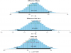
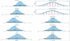
Figure 2. Visual synopsis of the results of a Bayesian parameter estimation via MCMC simulations for the difference between means for experimental condition V00 versus V01 with associated 95% HDIs and a ROPEs ranging from [-0.1,0.1], respectively.
Left panel: Posterior distribution of the means per experimental condition (i.e., V00 and V01; n=62) with associated 95% HDI (Bayesian posterior high density credible interval); the associated standard deviations (σ1 and σ2) with their associated 95% HDIs, and the Gaussianity parameter ν with its associated 95% HDI.
Upper right panel: Posterior predictive plots for the difference between means per experimental condition (n=62). Curves were produced by selecting random steps in the Markov chain and plotting the t-distribution (with the corresponding values of μ, σ and ν for that step). In total n=30 representative t-distributions are superimposed on the histogram of the actual empirical dataset.
Lower right panel: The difference between means with its associated ROPE ranging from [-0.1,0.1] and 95% HDI; the standard deviation of the a posteriori estimated difference and the corresponding effect size δ with its associated ROPE [-0.1,0.1] and 95% HDI.
References
Hastings, W. K. (1970). Monte Carlo sampling methods using Markov chains and their applications. Biometrika, 57(1), 97–109.
Kruschke, J. K., & Liddell, T. M. (2018). The Bayesian New Statistics: Hypothesis testing, estimation, meta-analysis, and power analysis from a Bayesian perspective. Psychonomic Bulletin & Review, 25(1), 178–206.
#clears all of R's memory
rm(list=ls())
# Get the functions loaded into R's working memory
# The function can also be downloaded from the following URL: # http://irrational-decisions.com/?page_id=1996
source("BEST.R")
#download data from server
dataexp2 <-
read.table("http://www.irrational-decisions.com/phd-thesis/dataexp2.txt",
header=TRUE, sep="", na.strings="NA", dec=".", strip.white=TRUE)
# Specify data as vectors
y1 = c(dataexp2$v00)
y2 = c(dataexp2$v01)
# Run the Bayesian analysis using the default broad priors described by Kruschke (2013)
mcmcChain = BESTmcmc( y1 , y2 , priorOnly=FALSE ,
numSavedSteps=12000 , thinSteps=1 , showMCMC=TRUE )
postInfo = BESTplot( y1 , y2 , mcmcChain , ROPEeff=c(-0.1,0.1) )

#The function “BEST.R” can be downloaded from the CRAN (Comprehensive R Archive Network) repository under https://cran.r-project.org/web/packages/BEST/index.html
Useful software
The Bugs project
(University of Cambridge)
https://www.mrc-bsu.cam.ac.uk/software/bugs/embed/
The BUGS (Bayesian inference Using Gibbs Sampling) project is concerned with flexible software for the Bayesian analysis of complex statistical models using Markov chain Monte Carlo (MCMC) methods. The project began in 1989 in the MRC Biostatistics Unit, Cambridge, and led initially to the `Classic’ BUGS program, and then onto the WinBUGS software developed jointly with the Imperial College School of Medicine at St Mary’s, London. Developments were later focused on the OpenBUGS, an open source equivalent of WinBUGS.
JAGS:
http://mcmc-jags.sourceforge.net/
JAGS is Just Another Gibbs Sampler. It is a program for analysis of Bayesian hierarchical models using Markov Chain Monte Carlo (MCMC) simulation not wholly unlike BUGS. JAGS was written with three aims in mind:
- To have a cross-platform engine for the BUGS language
- To be extensible, allowing users to write their own functions, distributions and samplers.
- To be a platform for experimentation with ideas in Bayesian modelling
JAGS is licensed under the GNU General Public License version 2. You may freely modify and redistribute it under certain conditions (see the file COPYING for details).
BEST:
http://www.indiana.edu/~kruschke/BEST/
Bayesian estimation for two groups provides complete distributions of credible values for the effect size, group means and their difference, standard deviations and their difference, and the normality of the data. The method handles outliers. The decision rule can accept the null value (unlike traditional t tests) when certainty in the estimate is high (unlike Bayesian model comparison using Bayes factors). The method also yields precise estimates of statistical power for various research goals. The software and programs are free, and run on Macintosh, Linux, and Windows platforms.
Pandoc
Pandochttps://pandoc.org/
If you need to convert files from one markup format into another, pandoc is your swiss-army knife. Pandoc can convert documents in (several dialects of) Markdown, reStructuredText, textile, HTML,DocBook, LaTeX, MediaWiki markup, TWiki markup, TikiWiki markup, Creole 1.0, Vimwiki markup,OPML, Emacs Org-Mode, Emacs Muse, txt2tags, Microsoft Word docx, LibreOffice ODT, EPUB, or Haddock markup.