Results of Bayesian analyses can be utilised for future research in the sense of Dennis Lindley’s motto: “Today’s posterior is tomorrow’s prior” (Lindley, 1972), or as Richard Feynman put it “Yesterday’s sensation is today’s calibration” to which Valentine Telegdi added“…and tomorrow’s background”.


At the conceptual meta level, the primary difference between the frequentists and the Bayesian account is that the former treats data as random and parameters as fixed and the latter regards data as fixed and unknown parameters as random.
A Bayes Factor can range from 0 to ∞ and a value of 1 denotes equivalent support for both competing hypotheses. Moreover, LogBF10 can be expressed as a logarithm ranging from -∞ to ∞. A BF of 0 denotes equal support for H0 and H1.
“The prior distribution is a key part of Bayesian inference and represents the information about an uncertain parameter that is combined with the probability distribution of new data to yield the posterior distribution, which in turn is used for future inferences and decisions.” (Gelman, 2006, p. 1634)
In a seminal paper entitled “Inference, method, and decision: towards a Bayesian philosophy of science” Rosenkrantz (Rosenkrantz, 1980, p. 485) discusses the Popperian concept of verisimilitude (truthlikeness) w.r.t. Bayesian decision making and develops a persuasive cogent argument in favour of diffuse priors (i.e., C-systems with a low λ). In a related publication he states: “If your prior is heavily concentrated about the true value (which amounts to a ‘lucky guess’ in the absence of pertinent data), you stand to be slightly closer to the truth after sampling than someone who adopts a diffuse prior, your advantage dissipating rapidly with sample size. If, however, your initial estimate is in error, you will be farther from the truth after sampling, and if the error is substantial, you will be much farther from the truth. I can express this by saying that a diffuse prior is a better choice at ‘almost all’ values of [q1] or, better, that it semi~dominates any highly peaked (or ‘opinionated’) prior. In practice, a diffuse prior never does much worse than a peaked one and ‘generally’ does much better…” (1946)
data(ToothGrowth)

## Example plot from ?ToothGrowth

coplot(len ~ dose | supp, data = ToothGrowth, panel = panel.smooth,
       xlab = "ToothGrowth data: length vs dose, given type of supplement")
## Treat dose as a factor
ToothGrowth$dose = factor(ToothGrowth$dose)
levels(ToothGrowth$dose) = c("Low", "Medium", "High")

summary(aov(len ~ supp*dose, data=ToothGrowth))


#install.packages("xtable")
library(xtable)
xtable(x, caption = NULL, label = NULL, align = NULL, digits = NULL,
       display = NULL, auto = FALSE, ...)

print(xtable(d), type="html")
print(xtable(d), type="latex") # anova table to latex
#https://cran.r-project.org/web/packages/xtable/index.html
#https://rmarkdown.rstudio.com/
data(ToothGrowth)

# model log2 of dose instead of dose directly
ToothGrowth$dose = log2(ToothGrowth$dose)

# Classical analysis for comparison
lmToothGrowth <- lm(len ~ supp + dose + supp:dose, data=ToothGrowth)
summary(lmToothGrowth)
x<- (1:5)
y<- (1:111)
pdf(file=file.choose())
hist(x)
plot(x, type='o')
dev.off()
Notes
file.choose() is a very handy command which saves the work associated with defining absolute and relative paths which can be quite cumbersome.
list.files for non-interactive selection.
choose.files for selecting multiple files interactively.
More
https://www.rdocumentation.org/packages/base/versions/3.5.2/topics/file.choose
# http://wiki.math.yorku.ca/index.php/VR4:_Chapter_1_summary
x <- seq( 1, 20, 0.5)   # sequence from 1 to 20 by 0.5
x                       # print it
w <- 1 + x/2            # a weight vector
y <- x + w*rnorm(x)     # generate y with standard deviations
                          #    equal to w

dum <- data.frame( x, y, w )     # make a data frame of 3 columns
dum                     # typing it's name shows the object
rm( x, y, w )           # remove the original variables


fm <- lm ( y ~ x, data = dum)   # fit a simple linear regression (between x and y)
summary( fm )                   # and look at the analysis


fm1 <- lm( y ~ x, data = dum, weight = 1/w^2 )  # a weighted regression
summary(fm1)

lrf <- loess( y ~ x, dum)    # a smooth regression curve using a
                               #   modern local regression function
attach( dum )                # make the columns in the data frame visible
                               #   as variables (Note: before this command, typing x and
                               #   y would yield errors)
plot( x, y)                  # a standard scatterplot to which we will
                               #   fit regression curves
lines( spline( x, fitted (lrf)), col = 2)  # add in the local regression using spline
                                             #  interpolation between calculated
                                             #  points
abline(0, 1, lty = 3, col = 3)    # add in the true regression line (lty=3: read line type=dotted;
                                    #   col=3: read colour=green; type "?par" for details)
abline(fm, col = 4)               # add in the unweighted regression line
abline(fm1, lty = 4, col = 5)     # add in the weighted regression line
plot( fitted(fm), resid(fm),
       xlab = "Fitted Values",
       ylab = "Residuals")          # a standard regression diagnostic plot
                                    # to check for heteroscedasticity.
                                    # The data were generated from a
                                    # heteroscedastic process. Can you see
                                    # it from this plot?
qqnorm( resid(fm) )               # Normal scores to check for skewness,
                                    #   kurtosis and outliers.  How would you
                                    #   expect heteroscedasticity to show up?
search()                          # Have a look at the search path
detach()                          # Remove the data frame from the search path
search()                          # Have another look. How did it change?
rm(fm, fm1, lrf, dum)             # Clean up (this is not that important in R
                                    #    for reasons we will understand later)


library(rgl)
rgl.open()
rgl.bg(col='white')
x <- sort(rnorm(1000))
y <- rnorm(1000)
z1 <- atan2(x,y)
z <- rnorm(1000) + atan2(x, y)
plot3d(x, y, z1, col = rainbow(1000), size = 2)
bbox3d()
skew(x, na.rm = TRUE)
kurtosi(x, na.rm = TRUE)

#x A data.frame or matrix
#na.rm how to treat missing data

## The function is currently defined as
function (x, na.rm = TRUE)
{
    if (length(dim(x)) == 0) {
        if (na.rm) {
            x <- x[!is.na(x)]
        			}

        mx <- mean(x)
         sdx <- sd(x,na.rm=na.rm)
        kurt <- sum((x - mx)^4)/(length(x) * sd(x)^4)  -3
        } else {

    kurt <- rep(NA,dim(x)[2])
    mx <- colMeans(x,na.rm=na.rm)
     sdx <- sd(x,na.rm=na.rm)
    for (i in 1:dim(x)[2]) {
    kurt[i] <- sum((x[,i] - mx[i])^4,  na.rm = na.rm)/((length(x[,i]) - sum(is.na(x[,i]))) * sdx[i]^4)  -3
            }
    }
    return(kurt)
  }
#https://richarddmorey.github.io/BayesFactor/
bf = ttestBF(x = diffScores)
## Equivalently:
## bf = ttestBF(x = sleep$extra[1:10],y=sleep$extra[11:20], paired=TRUE)
bf
Comment
ttestBF function, which performs the “JZS” t test described by Rouder, Speckman, Sun, Morey, and Iverson (2009).
#https://richarddmorey.github.io/BayesFactor/
chains2 = recompute(chains, iterations = 10000)
plot(chains2[,1:2])
Comment
The posterior function returns a object of type BFmcmc, which inherits the methods of the mcmc class from the coda package.
#https://richarddmorey.github.io/BayesFactor/
## Compute Bayes factor
bf = ttestBF(formula = weight ~ feed, data = chickwts)
bf
###
chains = posterior(bf, iterations = 10000)
plot(chains[,2])
#https://richarddmorey.github.io/BayesFactor/
## Bem's t statistics from four selected experiments
t = c(-.15, 2.39, 2.42, 2.43)
N = c(100, 150, 97, 99)
###
## Do analysis again, without nullInterval restriction
bf = meta.ttestBF(t=t, n1=N, rscale=1)

## Obtain posterior samples
chains = posterior(bf, iterations = 10000)
plot(chains)
Comment
ttestBF function, which performs the “JZS” t test described by Rouder, Speckman, Sun, Morey, and Iverson (2009).
## This source code is licensed under the FreeBSD license
## (c) 2013 Felix Schönbrodt

#' @title Plots a comparison of a sequence of priors for t test Bayes factors
#'
#' @details
#'
#'
#' @param ts A vector of t values
#' @param ns A vector of corresponding sample sizes
#' @param rs The sequence of rs that should be tested. r should run up to 2 (higher values are implausible; E.-J. Wagenmakers, personal communication, Aug 22, 2013)
#' @param labels Names for the studies (displayed in the facet headings)
#' @param dots Values of r's which should be marked with a red dot
#' @param plot If TRUE, a ggplot is returned. If false, a data frame with the computed Bayes factors is returned
#' @param sides If set to "two" (default), a two-sided Bayes factor is computed. If set to "one", a one-sided Bayes factor is computed. In this case, it is assumed that positive t values correspond to results in the predicted direction and negative t values to results in the unpredicted direction. For details, see Wagenmakers, E. J., & Morey, R. D. (2013). Simple relation between one-sided and two-sided Bayesian point-null hypothesis tests.
#' @param nrow Number of rows of the faceted plot.
#' @param forH1 Defines the direction of the BF. If forH1 is TRUE, BF > 1 speak in favor of H1 (i.e., the quotient is defined as H1/H0). If forH1 is FALSE, it's the reverse direction.
#'
#' @references
#'
#' Rouder, J. N., Speckman, P. L., Sun, D., Morey, R. D., & Iverson, G. (2009). Bayesian t-tests for accepting and rejecting the null hypothesis. Psychonomic Bulletin and Review, 16, 225-237.
#' Wagenmakers, E.-J., & Morey, R. D. (2013). Simple relation between one-sided and two-sided Bayesian point-null hypothesis tests. Manuscript submitted for publication
#' Wagenmakers, E.-J., Wetzels, R., Borsboom, D., Kievit, R. & van der Maas, H. L. J. (2011). Yes, psychologists must change the way they analyze their data: Clarifications for Bem, Utts, & Johnson (2011)

BFrobustplot <- function(
    ts, ns, rs=seq(0, 2, length.out=200), dots=1, plot=TRUE,
    labels=c(), sides="two", nrow=2, xticks=3, forH1=TRUE)
{
    library(BayesFactor)

    # compute one-sided p-values from ts and ns
    ps <- pt(ts, df=ns-1, lower.tail = FALSE)   # one-sided test

    # add the dots location to the sequences of r's
    rs <- c(rs, dots)

    res <- data.frame()
    for (r in rs) {

        # first: calculate two-sided BF
        B_e0 <- c()
        for (i in 1:length(ts))
            B_e0 <- c(B_e0, exp(ttest.tstat(t = ts[i], n1 = ns[i], rscale=r)$bf))

        # second: calculate one-sided BF
        B_r0 <- c() for (i in 1:length(ts)) { if (ts[i] > 0) {
                # correct direction
                B_r0 <- c(B_r0, (2 - 2*ps[i])*B_e0[i])
            } else {
                # wrong direction
                B_r0 <- c(B_r0, (1 - ps[i])*2*B_e0[i])
            }
        }

        res0 <- data.frame(t=ts, n=ns, BF_two=B_e0, BF_one=B_r0, r=r) if (length(labels) > 0) {
            res0$labels <- labels
            res0$heading <- factor(1:length(labels), labels=paste0(labels, "\n(t = ", ts, ", df = ", ns-1, ")"), ordered=TRUE)
        } else {
            res0$heading <- factor(1:length(ts), labels=paste0("t = ", ts, ", df = ", ns-1), ordered=TRUE)
        }
        res <- rbind(res, res0)
    }

    # define the measure to be plotted: one- or two-sided?
    res$BF <- res[, paste0("BF_", sides)]


    # Flip BF if requested
    if (forH1 == FALSE) {
        res$BF <- 1/res$BF
    }


    if (plot==TRUE) {
        library(ggplot2)
        p1 <- ggplot(res, aes(x=r, y=log(BF))) + geom_line() + facet_wrap(~heading, nrow=nrow) + theme_bw() + ylab("log(BF)")
        p1 <- p1 + geom_hline(yintercept=c(c(-log(c(30, 10, 3)), log(c(3, 10, 30)))), linetype="dotted", color="darkgrey")
        p1 <- p1 + geom_hline(yintercept=log(1), linetype="dashed", color="darkgreen")

        # add the dots
        p1 <- p1 + geom_point(data=res[res$r %in% dots,], aes(x=r, y=log(BF)), color="red", size=2)

        # add annotation
        p1 <- p1 + annotate("text", x=max(rs)*1.8, y=-2.85, label=paste0("Strong~H[", ifelse(forH1==TRUE,0,1), "]"), hjust=1, vjust=.5, size=3, color="black", parse=TRUE)
        p1 <- p1 + annotate("text", x=max(rs)*1.8, y=-1.7 , label=paste0("Moderate~H[", ifelse(forH1==TRUE,0,1), "]"), hjust=1, vjust=.5, size=3, color="black", parse=TRUE)
        p1 <- p1 + annotate("text", x=max(rs)*1.8, y=-.55 , label=paste0("Anectodal~H[", ifelse(forH1==TRUE,0,1), "]"), hjust=1, vjust=.5, size=3, color="black", parse=TRUE)
        p1 <- p1 + annotate("text", x=max(rs)*1.8, y=2.86 , label=paste0("Strong~H[", ifelse(forH1==TRUE,1,0), "]"), hjust=1, vjust=.5, size=3, color="black", parse=TRUE)
        p1 <- p1 + annotate("text", x=max(rs)*1.8, y=1.7  , label=paste0("Moderate~H[", ifelse(forH1==TRUE,1,0), "]"), hjust=1, vjust=.5, size=3, color="black", parse=TRUE)
        p1 <- p1 + annotate("text", x=max(rs)*1.8, y=.55  , label=paste0("Anectodal~H[", ifelse(forH1==TRUE,1,0), "]"), hjust=1, vjust=.5, vjust=.5, size=3, color="black", parse=TRUE)

        # set scale ticks
        p1 <- p1 + scale_y_continuous(breaks=c(c(-log(c(30, 10, 3)), 0, log(c(3, 10, 30)))), labels=c("-log(30)", "-log(10)", "-log(3)", "log(1)", "log(3)", "log(10)", "log(30)"))
        p1 <- p1 + scale_x_continuous(breaks=seq(min(rs), max(rs), length.out=xticks))

        return(p1)
    } else {
        return(res)
    }
}
References
Rouder, J. N., Speckman, P. L., Sun, D., Morey, R. D., & Iverson, G. (2009). Bayesian t-tests for accepting and rejecting the null hypothesis. Psychonomic Bulletin and Review, 16, 225-237
#https://jimgrange.wordpress.com/2015/11/27/animating-robustness-check-of-bayes-factor-priors/
### plots of prior robustness check

# gif created from PNG plots using http://gifmaker.me/

# clear R's memory
rm(list = ls())

# load the Bayes factor package
library(BayesFactor)

# set working directory (will be used to save files here, so make sure
# this is where you want to save your plots!)
setwd <- "D:/Work//Blog_YouTube code//Blog/Prior Robust Visualisation/plots"

#------------------------------------------------------------------------------
### declare some variables for the analysis

# what is the t-value for the data?
tVal <- 3.098

# how many points in the prior should be explored?
nPoints <- 1000

# what Cauchy rates should be explored?
cauchyRates <- seq(from = 0.01, to = 1.5, length.out = nPoints)

# what effect sizes should be plotted?
effSize <- seq(from = -2, to = 2, length.out = nPoints)

# get the Bayes factor for each prior value
bayesFactors <- sapply(cauchyRates, function(x)
  exp(ttest.tstat(t = tVal, n1 = 76, rscale = x)[['bf']]))
#------------------------------------------------------------------------------

#------------------------------------------------------------------------------
### do the plotting

# how many plots do we want to produce?
nPlots <- 50
plotWidth <- round(seq(from = 1, to = nPoints, length.out = nPlots), 0)

# loop over each plot
for(i in plotWidth){

  # set up the file
  currFile <- paste(getwd(), "/plot_", i, ".png", sep = "")

  # initiate the png file
  png(file = currFile, width = 1200, height = 1000, res = 200)

  # change the plotting window so plots appear side-by-side
  par(mfrow = c(1, 2))

  #----
  # do the prior density plot
  d <- dcauchy(effSize, scale = cauchyRates[i])
  plot(effSize, d, type = "l", ylim = c(0, 5), xlim = c(-2, 2),
       ylab = "Density", xlab = "Effect Size (d)", lwd = 2, col = "gray48",
       main = paste("Rate (r) = ", round(cauchyRates[i], 3), sep = ""))

  #-----
  # do the Bayes factor plot
  plot(cauchyRates, bayesFactors, type = "l", lwd = 2, col = "gray48",
       ylim = c(0, max(bayesFactors)), xaxt = "n",
                xlab = "Cauchy Prior Width (r)", ylab = "Bayes Factor (10)")
  abline(h = 0, lwd = 1)
  abline(h = 6, col = "black", lty = 2, lwd = 2)
  axis(1, at = seq(0, 1.5, 0.25))

  # add the BF at the default Cauchy point
  points(0.707, 9.97, col = "black", cex = 1.5, pch = 21, bg = "red")

  # add the BF for the Cauchy prior currently being plotted
  points(cauchyRates[i], bayesFactors[i], col = "black", pch = 21, cex = 1.3,
         bg = "cyan")

  # add legend
  legend(x = 0.25, y = 3, legend = c("r = 0.707", paste("r = ",
                                                      round(cauchyRates[i], 3),
                                                            sep = "")),
         pch = c(21, 21), lty = c(NA, NA), lwd = c(NA, NA), pt.cex = c(1, 1),
         col = c("black", "black"), pt.bg = c("red", "cyan"), bty = "n")

  # save the current plot
  dev.off()

}
#------------------------------------------------------------------------------
skew(x, na.rm = TRUE)
kurtosi(x, na.rm = TRUE)

#x A data.frame or matrix
#na.rm how to treat missing data

## The function is currently defined as
function (x, na.rm = TRUE)
{
    if (length(dim(x)) == 0) {
        if (na.rm) {
            x <- x[!is.na(x)]
        			}

        mx <- mean(x)
         sdx <- sd(x,na.rm=na.rm)
        kurt <- sum((x - mx)^4)/(length(x) * sd(x)^4)  -3
        } else {

    kurt <- rep(NA,dim(x)[2])
    mx <- colMeans(x,na.rm=na.rm)
     sdx <- sd(x,na.rm=na.rm)
    for (i in 1:dim(x)[2]) {
    kurt[i] <- sum((x[,i] - mx[i])^4,  na.rm = na.rm)/((length(x[,i]) - sum(is.na(x[,i]))) * sdx[i]^4)  -3
            }
    }
    return(kurt)
  }
#https://richarddmorey.github.io/BayesFactor/
data(ToothGrowth)

## Example plot from ?ToothGrowth

coplot(len ~ dose | supp, data = ToothGrowth, panel = panel.smooth,
       xlab = "ToothGrowth data: length vs dose, given type of supplement")
bf = anovaBF(len ~ supp*dose, data=ToothGrowth)
bf
plot(bf[3:4] / bf[2])

#reduce number of comparisons (alpha inflation)
bf = anovaBF(len ~ supp*dose, data=ToothGrowth, whichModels="top")
bf
bfMainEffects = lmBF(len ~ supp + dose, data = ToothGrowth)
bfInteraction = lmBF(len ~ supp + dose + supp:dose, data = ToothGrowth)
## Compare the two models
bf = bfInteraction / bfMainEffects
bf
##
newbf = recompute(bf, iterations = 500000)
newbf

# posterior function
## Sample from the posterior of the full model
chains = posterior(bfInteraction, iterations = 10000)
## 1:13 are the only "interesting" parameters
summary(chains[,1:13])
#lot posterior of selected effects
plot(chains[,4:6])
Comment
Reduce number of comparisons by specifyig the xact model of interest a priori.
# MODIFIED FROM BEST.R FOR ONE GROUP INSTEAD OF TWO.
# Version of Dec 02, 2015.
# John K. Kruschke
# johnkruschke@gmail.com
# http://www.indiana.edu/~kruschke/BEST/
#
# This program is believed to be free of errors, but it comes with no guarantee!
# The user bears all responsibility for interpreting the results.
# Please check the webpage above for updates or corrections.
#
### ***************************************************************
### ******** SEE FILE BEST1Gexample.R FOR INSTRUCTIONS ************
### ***************************************************************

source("openGraphSaveGraph.R") # graphics functions for Windows, Mac OS, Linux

BEST1Gmcmc = function( y , numSavedSteps=100000, thinSteps=1, showMCMC=FALSE) {
  # This function generates an MCMC sample from the posterior distribution.
  # Description of arguments:
  # showMCMC is a flag for displaying diagnostic graphs of the chains.
  #    If F (the default), no chain graphs are displayed. If T, they are.

  require(rjags)

  #------------------------------------------------------------------------------
  # THE MODEL.
  modelString = "
  model {
    for ( i in 1:Ntotal ) {
      y[i] ~ dt( mu , tau , nu )
    }
    mu ~ dnorm( muM , muP )
    tau <- 1/pow( sigma , 2 )
    sigma ~ dunif( sigmaLow , sigmaHigh )
    nu ~ dexp(1/30)
}
  " # close quote for modelString
  # Write out modelString to a text file
  writeLines( modelString , con="BESTmodel.txt" )

  #------------------------------------------------------------------------------
  # THE DATA.
  # Load the data:
  Ntotal = length(y)
  # Specify the data in a list, for later shipment to JAGS:
  dataList = list(
    y = y ,
    Ntotal = Ntotal ,
    muM = mean(y) ,
    muP = 0.000001 * 1/sd(y)^2 ,
    sigmaLow = sd(y) / 1000 ,
    sigmaHigh = sd(y) * 1000
  )

  #------------------------------------------------------------------------------
  # INTIALIZE THE CHAINS.
  # Initial values of MCMC chains based on data:
  mu = mean(y)
  sigma = sd(y)
  # Regarding initial values in next line: (1) sigma will tend to be too big if
  # the data have outliers, and (2) nu starts at 5 as a moderate value. These
  # initial values keep the burn-in period moderate.
  initsList = list( mu = mu , sigma = sigma , nu = 5 )

  #------------------------------------------------------------------------------
  # RUN THE CHAINS

  parameters = c( "mu" , "sigma" , "nu" )     # The parameters to be monitored
  adaptSteps = 500               # Number of steps to "tune" the samplers
  burnInSteps = 1000
  nChains = 3
  nIter = ceiling( ( numSavedSteps * thinSteps ) / nChains )
  # Create, initialize, and adapt the model:
  jagsModel = jags.model( "BESTmodel.txt" , data=dataList , inits=initsList ,
                          n.chains=nChains , n.adapt=adaptSteps )
  # Burn-in:
  cat( "Burning in the MCMC chain...\n" )
  update( jagsModel , n.iter=burnInSteps )
  # The saved MCMC chain:
  cat( "Sampling final MCMC chain...\n" )
  codaSamples = coda.samples( jagsModel , variable.names=parameters ,
                              n.iter=nIter , thin=thinSteps )
  # resulting codaSamples object has these indices:
  #   codaSamples[[ chainIdx ]][ stepIdx , paramIdx ]

  #------------------------------------------------------------------------------
  # EXAMINE THE RESULTS
  if ( showMCMC ) {
    openGraph(width=7,height=7)
    autocorr.plot( codaSamples[[1]] , ask=FALSE )
    show( gelman.diag( codaSamples ) )
    effectiveChainLength = effectiveSize( codaSamples )
    show( effectiveChainLength )
  }

  # Convert coda-object codaSamples to matrix object for easier handling.
  # But note that this concatenates the different chains into one long chain.
  # Result is mcmcChain[ stepIdx , paramIdx ]
  mcmcChain = as.matrix( codaSamples )
  return( mcmcChain )

} # end function BESTmcmc

#==============================================================================

BEST1Gplot = function( y , mcmcChain , compValm=0.0 , ROPEm=NULL ,
                       compValsd=NULL , ROPEsd=NULL ,
                       ROPEeff=NULL , showCurve=FALSE , pairsPlot=FALSE ) {
  # This function plots the posterior distribution (and data).
  # Description of arguments:
  # y is the data vector.
  # mcmcChain is a list of the type returned by function BEST1G.
  # compValm is hypothesized mean for comparing with estimated mean.
  # ROPEm is a two element vector, such as c(-1,1), specifying the limit
  #   of the ROPE on the mean.
  # ROPEsd is a two element vector, such as c(14,16), specifying the limit
  #   of the ROPE on the difference of standard deviations.
  # ROPEeff is a two element vector, such as c(-1,1), specifying the limit
  #   of the ROPE on the effect size.
  # showCurve is TRUE or FALSE and indicates whether the posterior should
  #   be displayed as a histogram (by default) or by an approximate curve.
  # pairsPlot is TRUE or FALSE and indicates whether scatterplots of pairs
  #   of parameters should be displayed.
  mu = mcmcChain[,"mu"]
  sigma = mcmcChain[,"sigma"]
  nu = mcmcChain[,"nu"]

  if ( pairsPlot ) {
    # Plot the parameters pairwise, to see correlations:
    openGraph(width=7,height=7)
    nPtToPlot = 1000
    plotIdx = floor(seq(1,length(mu),by=length(mu)/nPtToPlot))
    panel.cor = function(x, y, digits=2, prefix="", cex.cor, ...) {
      usr = par("usr"); on.exit(par(usr))
      par(usr = c(0, 1, 0, 1))
      r = (cor(x, y))
      txt = format(c(r, 0.123456789), digits=digits)[1]
      txt = paste(prefix, txt, sep="")
      if(missing(cex.cor)) cex.cor <- 0.8/strwidth(txt)
      text(0.5, 0.5, txt, cex=1.25 ) # was cex=cex.cor*r
    }
    pairs( cbind( mu , sigma , log10(nu) )[plotIdx,] ,
           labels=c( expression(mu) ,
                     expression(sigma) ,
                     expression(log10(nu)) ) ,
           lower.panel=panel.cor , col="skyblue" )
  }

  # Define matrix for storing summary info:
  summaryInfo = NULL

  source("plotPost.R")
  # Set up window and layout:
  openGraph(width=6.0,height=5.0)
  layout( matrix( c(3,3,4,4,5,5, 1,1,1,1,2,2) , nrow=6, ncol=2 , byrow=FALSE ) )
  par( mar=c(3.5,3.5,2.5,0.5) , mgp=c(2.25,0.7,0) )

  # Select thinned steps in chain for plotting of posterior predictive curves:
  chainLength = NROW( mcmcChain )
  nCurvesToPlot = 30
  stepIdxVec = seq( 1 , chainLength , floor(chainLength/nCurvesToPlot) )
  xRange = range( y )
  xLim = c( xRange[1]-0.1*(xRange[2]-xRange[1]) ,
            xRange[2]+0.1*(xRange[2]-xRange[1]) )
  xVec = seq( xLim[1] , xLim[2] , length=200 )
  maxY = max( dt( 0 , df=max(nu[stepIdxVec]) ) / min(sigma[stepIdxVec]) )
  # Plot data y and smattering of posterior predictive curves:
  stepIdx = 1
  plot( xVec , dt( (xVec-mu[stepIdxVec[stepIdx]])/sigma[stepIdxVec[stepIdx]] ,
                   df=nu[stepIdxVec[stepIdx]] )/sigma[stepIdxVec[stepIdx]] ,
        ylim=c(0,maxY) , cex.lab=1.75 ,
        type="l" , col="skyblue" , lwd=1 , xlab="y" , ylab="p(y)" ,
        main="Data w. Post. Pred." )
  for ( stepIdx in 2:length(stepIdxVec) ) {
    lines(xVec, dt( (xVec-mu[stepIdxVec[stepIdx]])/sigma[stepIdxVec[stepIdx]] ,
                    df=nu[stepIdxVec[stepIdx]] )/sigma[stepIdxVec[stepIdx]] ,
          type="l" , col="skyblue" , lwd=1 )
  }
  histBinWd = median(sigma)/2
  histCenter = mean(mu)
  histBreaks = sort( c( seq( histCenter-histBinWd/2 , min(xVec)-histBinWd/2 ,
                             -histBinWd ),
                        seq( histCenter+histBinWd/2 , max(xVec)+histBinWd/2 ,
                             histBinWd ) , xLim ) )
  histInfo = hist( y , plot=FALSE , breaks=histBreaks )
  yPlotVec = histInfo$density
  yPlotVec[ yPlotVec==0.0 ] = NA
  xPlotVec = histInfo$mids
  xPlotVec[ yPlotVec==0.0 ] = NA
  points( xPlotVec , yPlotVec , type="h" , lwd=3 , col="red" )
  text( max(xVec) , maxY , bquote(N==.(length(y))) , adj=c(1.1,1.1) )

  # Plot posterior distribution of parameter nu:
  paramInfo = plotPost( log10(nu) , col="skyblue" , # breaks=30 ,
                       showCurve=showCurve ,
                       xlab=bquote("log10("*nu*")") , cex.lab = 1.75 , showMode=TRUE ,
                       main="Normality" ) #  (<0.7 suggests kurtosis)
  summaryInfo = rbind( summaryInfo , paramInfo )
  rownames(summaryInfo)[NROW(summaryInfo)] = "log10(nu)"

  # Plot posterior distribution of parameters mu1, mu2, and their difference:
  xlim = range( c( mu , compValm ) )
  paramInfo = plotPost( mu ,  xlim=xlim , cex.lab = 1.75 , ROPE=ROPEm ,
                       showCurve=showCurve , compVal = compValm ,
                       xlab=bquote(mu) , main=paste("Mean") ,
                       col="skyblue" )
  summaryInfo = rbind( summaryInfo , paramInfo )
  rownames(summaryInfo)[NROW(summaryInfo)] = "mu"

  # Plot posterior distribution of sigma:
  xlim=range( sigma )
  paramInfo = plotPost( sigma ,  xlim=xlim , cex.lab = 1.75 , ROPE=ROPEsd ,
                       showCurve=showCurve , compVal=compValsd ,
                       xlab=bquote(sigma) , main=paste("Std. Dev.") ,
                       col="skyblue" , showMode=TRUE )
  summaryInfo = rbind( summaryInfo , paramInfo )
  rownames(summaryInfo)[NROW(summaryInfo)] = "sigma"

  # Plot of estimated effect size:
  effectSize = ( mu - compValm ) / sigma
  paramInfo = plotPost( effectSize , compVal=0 ,  ROPE=ROPEeff ,
                       showCurve=showCurve ,
                       xlab=bquote( (mu-.(compValm)) / sigma ),
                       showMode=TRUE , cex.lab=1.75 , main="Effect Size" , col="skyblue" )
  summaryInfo = rbind( summaryInfo , paramInfo )
  rownames(summaryInfo)[NROW(summaryInfo)] = "effSz"

  return( summaryInfo )

  } # end of function BEST1Gplot

#==============================================================================
# MODIFIED 2015 DEC 02.
# John K. Kruschke
# johnkruschke@gmail.com
# http://www.indiana.edu/~kruschke/BEST/
#
# This program is believed to be free of errors, but it comes with no guarantee!
# The user bears all responsibility for interpreting the results.
# Please check the webpage above for updates or corrections.
#
### ***************************************************************
### ******** SEE FILE BESTexample.R FOR INSTRUCTIONS **************
### ***************************************************************

# Load various essential functions:
source("DBDA2E-utilities.R")

BESTmcmc = function( y1 , y2 ,
                     priorOnly=FALSE , showMCMC=FALSE ,
                     numSavedSteps=20000 , thinSteps=1 ,
                     mu1PriorMean = mean(c(y1,y2)) ,
                     mu1PriorSD = sd(c(y1,y2))*5 ,
                     mu2PriorMean = mean(c(y1,y2)) ,
                     mu2PriorSD = sd(c(y1,y2))*5 ,
                     sigma1PriorMode = sd(c(y1,y2)) ,
                     sigma1PriorSD = sd(c(y1,y2))*5 ,
                     sigma2PriorMode = sd(c(y1,y2)) ,
                     sigma2PriorSD = sd(c(y1,y2))*5 ,
                     nuPriorMean = 30 ,
                     nuPriorSD = 30 ,
                     runjagsMethod=runjagsMethodDefault ,
                     nChains=nChainsDefault ) {
  # This function generates an MCMC sample from the posterior distribution.
  # Description of arguments:
  # showMCMC is a flag for displaying diagnostic graphs of the chains.
  #    If F (the default), no chain graphs are displayed. If T, they are.

  #------------------------------------------------------------------------------
  # THE DATA.
  # Load the data:
  y = c( y1 , y2 ) # combine data into one vector
  x = c( rep(1,length(y1)) , rep(2,length(y2)) ) # create group membership code
  Ntotal = length(y)
  # Specify the data and prior constants in a list, for later shipment to JAGS:
  if ( priorOnly ) {
    dataList = list(
      #  y = y ,
      x = x ,
      Ntotal = Ntotal ,
      mu1PriorMean = mu1PriorMean ,
      mu1PriorSD = mu1PriorSD ,
      mu2PriorMean = mu2PriorMean ,
      mu2PriorSD = mu2PriorSD ,
      Sh1 = gammaShRaFromModeSD( mode=sigma1PriorMode ,
                                 sd=sigma1PriorSD )$shape ,
      Ra1 = gammaShRaFromModeSD( mode=sigma1PriorMode ,
                                 sd=sigma1PriorSD )$rate ,
      Sh2 = gammaShRaFromModeSD( mode=sigma2PriorMode ,
                                 sd=sigma2PriorSD )$shape ,
      Ra2 = gammaShRaFromModeSD( mode=sigma2PriorMode ,
                                 sd=sigma2PriorSD )$rate ,
      ShNu = gammaShRaFromMeanSD( mean=nuPriorMean , sd=nuPriorSD )$shape ,
      RaNu = gammaShRaFromMeanSD( mean=nuPriorMean , sd=nuPriorSD )$rate
    )
  } else {
    dataList = list(
      y = y ,
      x = x ,
      Ntotal = Ntotal ,
      mu1PriorMean = mu1PriorMean ,
      mu1PriorSD = mu1PriorSD ,
      mu2PriorMean = mu2PriorMean ,
      mu2PriorSD = mu2PriorSD ,
      Sh1 = gammaShRaFromModeSD( mode=sigma1PriorMode ,
                                 sd=sigma1PriorSD )$shape ,
      Ra1 = gammaShRaFromModeSD( mode=sigma1PriorMode ,
                                 sd=sigma1PriorSD )$rate ,
      Sh2 = gammaShRaFromModeSD( mode=sigma2PriorMode ,
                                 sd=sigma2PriorSD )$shape ,
      Ra2 = gammaShRaFromModeSD( mode=sigma2PriorMode ,
                                 sd=sigma2PriorSD )$rate ,
      ShNu = gammaShRaFromMeanSD( mean=nuPriorMean , sd=nuPriorSD )$shape ,
      RaNu = gammaShRaFromMeanSD( mean=nuPriorMean , sd=nuPriorSD )$rate
    )
  }

  #----------------------------------------------------------------------------
  # THE MODEL.
  modelString = "
  model {
    for ( i in 1:Ntotal ) {
      y[i] ~ dt( mu[x[i]] , 1/sigma[x[i]]^2 , nu )
    }
    mu[1] ~ dnorm( mu1PriorMean , 1/mu1PriorSD^2 )  # prior for mu[1]
    sigma[1] ~ dgamma( Sh1 , Ra1 )     # prior for sigma[1]
    mu[2] ~ dnorm( mu2PriorMean , 1/mu2PriorSD^2 )  # prior for mu[2]
    sigma[2] ~ dgamma( Sh2 , Ra2 )     # prior for sigma[2]
    nu ~ dgamma( ShNu , RaNu ) # prior for nu
  }
  " # close quote for modelString
  # Write out modelString to a text file
  writeLines( modelString , con="BESTmodel.txt" )

  #------------------------------------------------------------------------------
  # INTIALIZE THE CHAINS.
  # Initial values of MCMC chains based on data:
  mu = c( mean(y1) , mean(y2) )
  sigma = c( sd(y1) , sd(y2) )
  # Regarding initial values in next line: (1) sigma will tend to be too big if
  # the data have outliers, and (2) nu starts at 5 as a moderate value. These
  # initial values keep the burn-in period moderate.
  initsList = list( mu = mu , sigma = sigma , nu = 5 )

  #------------------------------------------------------------------------------
  # RUN THE CHAINS

  parameters = c( "mu" , "sigma" , "nu" )     # The parameters to be monitored
  adaptSteps = 500               # Number of steps to "tune" the samplers
  burnInSteps = 1000

  runJagsOut <- run.jags( method=runjagsMethod , model="BESTmodel.txt" , monitor=parameters , data=dataList , inits=initsList , n.chains=nChains , adapt=adaptSteps , burnin=burnInSteps , sample=ceiling(numSavedSteps/nChains) , thin=thinSteps , summarise=FALSE , plots=FALSE ) codaSamples = as.mcmc.list( runJagsOut ) # resulting codaSamples object has these indices: # codaSamples[[ chainIdx ]][ stepIdx , paramIdx ] ## Original version, using rjags: # nChains = 3 # nIter = ceiling( ( numSavedSteps * thinSteps ) / nChains ) # # Create, initialize, and adapt the model: # jagsModel = jags.model( "BESTmodel.txt" , data=dataList , inits=initsList , # n.chains=nChains , n.adapt=adaptSteps ) # # Burn-in: # cat( "Burning in the MCMC chain...\n" ) # update( jagsModel , n.iter=burnInSteps ) # # The saved MCMC chain: # cat( "Sampling final MCMC chain...\n" ) # codaSamples = coda.samples( jagsModel , variable.names=parameters , # n.iter=nIter , thin=thinSteps ) #------------------------------------------------------------------------------ # EXAMINE THE RESULTS if ( showMCMC ) { for ( paramName in varnames(codaSamples) ) { diagMCMC( codaSamples , parName=paramName ) } } # Convert coda-object codaSamples to matrix object for easier handling. # But note that this concatenates the different chains into one long chain. # Result is mcmcChain[ stepIdx , paramIdx ] mcmcChain = as.matrix( codaSamples ) return( mcmcChain ) } # end function BESTmcmc #============================================================================== BESTsummary = function( y1 , y2 , mcmcChain ) { #source("HDIofMCMC.R") # in DBDA2E-utilities.R mcmcSummary = function( paramSampleVec , compVal=NULL ) { meanParam = mean( paramSampleVec ) medianParam = median( paramSampleVec ) dres = density( paramSampleVec ) modeParam = dres$x[which.max(dres$y)] hdiLim = HDIofMCMC( paramSampleVec ) if ( !is.null(compVal) ) { pcgtCompVal = ( 100 * sum( paramSampleVec > compVal )
                      / length( paramSampleVec ) )
    } else {
      pcgtCompVal=NA
    }
    return( c( meanParam , medianParam , modeParam , hdiLim , pcgtCompVal ) )
  }
  # Define matrix for storing summary info:
  summaryInfo = matrix( 0 , nrow=9 , ncol=6 , dimnames=list(
    PARAMETER=c( "mu1" , "mu2" , "muDiff" , "sigma1" , "sigma2" , "sigmaDiff" ,
                 "nu" , "nuLog10" , "effSz" ),
    SUMMARY.INFO=c( "mean" , "median" , "mode" , "HDIlow" , "HDIhigh" ,
                    "pcgtZero" )
  ) )
  summaryInfo[ "mu1" , ] = mcmcSummary( mcmcChain[,"mu[1]"] )
  summaryInfo[ "mu2" , ] = mcmcSummary( mcmcChain[,"mu[2]"] )
  summaryInfo[ "muDiff" , ] = mcmcSummary( mcmcChain[,"mu[1]"]
                                           - mcmcChain[,"mu[2]"] ,
                                           compVal=0 )
  summaryInfo[ "sigma1" , ] = mcmcSummary( mcmcChain[,"sigma[1]"] )
  summaryInfo[ "sigma2" , ] = mcmcSummary( mcmcChain[,"sigma[2]"] )
  summaryInfo[ "sigmaDiff" , ] = mcmcSummary( mcmcChain[,"sigma[1]"]
                                              - mcmcChain[,"sigma[2]"] ,
                                              compVal=0 )
  summaryInfo[ "nu" , ] = mcmcSummary( mcmcChain[,"nu"] )
  summaryInfo[ "nuLog10" , ] = mcmcSummary( log10(mcmcChain[,"nu"]) )

  N1 = length(y1)
  N2 = length(y2)
  effSzChain = ( ( mcmcChain[,"mu[1]"] - mcmcChain[,"mu[2]"] )
                 / sqrt( ( mcmcChain[,"sigma[1]"]^2
                           + mcmcChain[,"sigma[2]"]^2 ) / 2 ) )
  summaryInfo[ "effSz" , ] = mcmcSummary( effSzChain , compVal=0 )
  # Or, use sample-size weighted version:
  # effSz = ( mu1 - mu2 ) / sqrt( ( sigma1^2 *(N1-1) + sigma2^2 *(N2-1) )
  #                               / (N1+N2-2) )
  # Be sure also to change plot label in BESTplot function, below.
  return( summaryInfo )
}

#==============================================================================

BESTplot = function( y1 , y2 , mcmcChain , ROPEm=NULL , ROPEsd=NULL ,
                     ROPEeff=NULL , showCurve=FALSE , pairsPlot=FALSE ) {
  # This function plots the posterior distribution (and data).
  # Description of arguments:
  # y1 and y2 are the data vectors.
  # mcmcChain is a list of the type returned by function BTT.
  # ROPEm is a two element vector, such as c(-1,1), specifying the limit
  #   of the ROPE on the difference of means.
  # ROPEsd is a two element vector, such as c(-1,1), specifying the limit
  #   of the ROPE on the difference of standard deviations.
  # ROPEeff is a two element vector, such as c(-1,1), specifying the limit
  #   of the ROPE on the effect size.
  # showCurve is TRUE or FALSE and indicates whether the posterior should
  #   be displayed as a histogram (by default) or by an approximate curve.
  # pairsPlot is TRUE or FALSE and indicates whether scatterplots of pairs
  #   of parameters should be displayed.
  mu1 = mcmcChain[,"mu[1]"]
  mu2 = mcmcChain[,"mu[2]"]
  sigma1 = mcmcChain[,"sigma[1]"]
  sigma2 = mcmcChain[,"sigma[2]"]
  nu = mcmcChain[,"nu"]
  if ( pairsPlot ) {
    # Plot the parameters pairwise, to see correlations:
    openGraph(width=7,height=7)
    nPtToPlot = 1000
    plotIdx = floor(seq(1,length(mu1),by=length(mu1)/nPtToPlot))
    panel.cor = function(x, y, digits=2, prefix="", cex.cor, ...) {
      usr = par("usr"); on.exit(par(usr))
      par(usr = c(0, 1, 0, 1))
      r = (cor(x, y))
      txt = format(c(r, 0.123456789), digits=digits)[1]
      txt = paste(prefix, txt, sep="")
      if(missing(cex.cor)) cex.cor <- 0.8/strwidth(txt)
      text(0.5, 0.5, txt, cex=1.25 ) # was cex=cex.cor*r
    }
    pairs( cbind( mu1 , mu2 , sigma1 , sigma2 , log10(nu) )[plotIdx,] ,
           labels=c( expression(mu[1]) , expression(mu[2]) ,
                     expression(sigma[1]) , expression(sigma[2]) ,
                     expression(log10(nu)) ) ,
           lower.panel=panel.cor , col="skyblue" )
  }
  # source("plotPost.R") # in DBDA2E-utilities.R
  # Set up window and layout:
  openGraph(width=6.0,height=8.0)
  layout( matrix( c(4,5,7,8,3,1,2,6,9,10) , nrow=5, byrow=FALSE ) )
  par( mar=c(3.5,3.5,2.5,0.5) , mgp=c(2.25,0.7,0) )

  # Select thinned steps in chain for plotting of posterior predictive curves:
  chainLength = NROW( mcmcChain )
  nCurvesToPlot = 30
  stepIdxVec = seq( 1 , chainLength , floor(chainLength/nCurvesToPlot) )
  xRange = range( c(y1,y2) )
  if ( isTRUE( all.equal( xRange[2] , xRange[1] ) ) ) {
    meanSigma = mean( c(sigma1,sigma2) )
    xRange = xRange + c( -meanSigma , meanSigma )
  }
  xLim = c( xRange[1]-0.1*(xRange[2]-xRange[1]) ,
            xRange[2]+0.1*(xRange[2]-xRange[1]) )
  xVec = seq( xLim[1] , xLim[2] , length=200 )
  maxY = max( dt( 0 , df=max(nu[stepIdxVec]) ) /
                min(c(sigma1[stepIdxVec],sigma2[stepIdxVec])) )
  # Plot data y1 and smattering of posterior predictive curves:
  stepIdx = 1
  plot( xVec , dt( (xVec-mu1[stepIdxVec[stepIdx]])/sigma1[stepIdxVec[stepIdx]] ,
                   df=nu[stepIdxVec[stepIdx]] )/sigma1[stepIdxVec[stepIdx]] ,
        ylim=c(0,maxY) , cex.lab=1.75 ,
        type="l" , col="skyblue" , lwd=1 , xlab="y" , ylab="p(y)" ,
        main="Data Group 1 w. Post. Pred." )
  for ( stepIdx in 2:length(stepIdxVec) ) {
    lines(xVec, dt( (xVec-mu1[stepIdxVec[stepIdx]])/sigma1[stepIdxVec[stepIdx]] ,
                    df=nu[stepIdxVec[stepIdx]] )/sigma1[stepIdxVec[stepIdx]] ,
          type="l" , col="skyblue" , lwd=1 )
  }
  histBinWd = median(sigma1)/2
  histCenter = mean(mu1)
  histBreaks = sort( c( seq( histCenter-histBinWd/2 , min(xVec)-histBinWd/2 ,
                             -histBinWd ),
                        seq( histCenter+histBinWd/2 , max(xVec)+histBinWd/2 ,
                             histBinWd ) , xLim ) )
  histInfo = hist( y1 , plot=FALSE , breaks=histBreaks )
  yPlotVec = histInfo$density
  yPlotVec[ yPlotVec==0.0 ] = NA
  xPlotVec = histInfo$mids
  xPlotVec[ yPlotVec==0.0 ] = NA
  points( xPlotVec , yPlotVec , type="h" , lwd=3 , col="red" )
  text( max(xVec) , maxY , bquote(N[1]==.(length(y1))) , adj=c(1.1,1.1) )
  # Plot data y2 and smattering of posterior predictive curves:
  stepIdx = 1
  plot( xVec , dt( (xVec-mu2[stepIdxVec[stepIdx]])/sigma2[stepIdxVec[stepIdx]] ,
                   df=nu[stepIdxVec[stepIdx]] )/sigma2[stepIdxVec[stepIdx]] ,
        ylim=c(0,maxY) , cex.lab=1.75 ,
        type="l" , col="skyblue" , lwd=1 , xlab="y" , ylab="p(y)" ,
        main="Data Group 2 w. Post. Pred." )
  for ( stepIdx in 2:length(stepIdxVec) ) {
    lines(xVec, dt( (xVec-mu2[stepIdxVec[stepIdx]])/sigma2[stepIdxVec[stepIdx]] ,
                    df=nu[stepIdxVec[stepIdx]] )/sigma2[stepIdxVec[stepIdx]] ,
          type="l" , col="skyblue" , lwd=1 )
  }
  histBinWd = median(sigma2)/2
  histCenter = mean(mu2)
  histBreaks = sort( c( seq( histCenter-histBinWd/2 , min(xVec)-histBinWd/2 ,
                             -histBinWd ),
                        seq( histCenter+histBinWd/2 , max(xVec)+histBinWd/2 ,
                             histBinWd ) , xLim ) )
  histInfo = hist( y2 , plot=FALSE , breaks=histBreaks )
  yPlotVec = histInfo$density
  yPlotVec[ yPlotVec==0.0 ] = NA
  xPlotVec = histInfo$mids
  xPlotVec[ yPlotVec==0.0 ] = NA
  points( xPlotVec , yPlotVec , type="h" , lwd=3 , col="red" )
  text( max(xVec) , maxY , bquote(N[2]==.(length(y2))) , adj=c(1.1,1.1) )

  # Plot posterior distribution of parameter nu:
  histInfo = plotPost( log10(nu) , col="skyblue" , # breaks=30 ,
                       showCurve=showCurve ,
                       xlab=bquote("log10("*nu*")") , cex.lab = 1.75 ,
                       cenTend=c("mode","median","mean")[1] ,
                       main="Normality" ) #  (<0.7 suggests kurtosis)

  # Plot posterior distribution of parameters mu1, mu2, and their difference:
  xlim = range( c( mu1 , mu2 ) )
  histInfo = plotPost( mu1 ,  xlim=xlim , cex.lab = 1.75 ,
                       showCurve=showCurve ,
                       xlab=bquote(mu[1]) , main=paste("Group",1,"Mean") ,
                       col="skyblue" )
  histInfo = plotPost( mu2 ,  xlim=xlim , cex.lab = 1.75 ,
                       showCurve=showCurve ,
                       xlab=bquote(mu[2]) , main=paste("Group",2,"Mean") ,
                       col="skyblue" )
  histInfo = plotPost( mu1-mu2 , compVal=0 ,  showCurve=showCurve ,
                       xlab=bquote(mu[1] - mu[2]) , cex.lab = 1.75 , ROPE=ROPEm ,
                       main="Difference of Means" , col="skyblue" )

  # Plot posterior distribution of param's sigma1, sigma2, and their difference:
  xlim=range( c( sigma1 , sigma2 ) )
  histInfo = plotPost( sigma1 ,  xlim=xlim , cex.lab = 1.75 ,
                       showCurve=showCurve ,
                       xlab=bquote(sigma[1]) , main=paste("Group",1,"Std. Dev.") ,
                       col="skyblue" , cenTend=c("mode","median","mean")[1] )
  histInfo = plotPost( sigma2 ,  xlim=xlim , cex.lab = 1.75 ,
                       showCurve=showCurve ,
                       xlab=bquote(sigma[2]) , main=paste("Group",2,"Std. Dev.") ,
                       col="skyblue" , cenTend=c("mode","median","mean")[1] )
  histInfo = plotPost( sigma1-sigma2 ,
                       compVal=0 ,  showCurve=showCurve ,
                       xlab=bquote(sigma[1] - sigma[2]) , cex.lab = 1.75 ,
                       ROPE=ROPEsd ,
                       main="Difference of Std. Dev.s" , col="skyblue" ,
                       cenTend=c("mode","median","mean")[1] )

  # Plot of estimated effect size. Effect size is d-sub-a from
  # Macmillan & Creelman, 1991; Simpson & Fitter, 1973; Swets, 1986a, 1986b.
  effectSize = ( mu1 - mu2 ) / sqrt( ( sigma1^2 + sigma2^2 ) / 2 )
  histInfo = plotPost( effectSize , compVal=0 ,  ROPE=ROPEeff ,
                       showCurve=showCurve ,
                       xlab=bquote( (mu[1]-mu[2])
                                    /sqrt((sigma[1]^2 +sigma[2]^2 )/2 ) ),
                       cenTend=c("mode","median","mean")[1] , cex.lab=1.0 , main="Effect Size" ,
                       col="skyblue" )
  # Or use sample-size weighted version:
  # Hedges 1981; Wetzels, Raaijmakers, Jakab & Wagenmakers 2009.
  # N1 = length(y1)
  # N2 = length(y2)
  # effectSize = ( mu1 - mu2 ) / sqrt( ( sigma1^2 *(N1-1) + sigma2^2 *(N2-1) )
  #                                    / (N1+N2-2) )
  # Be sure also to change BESTsummary function, above.
  # histInfo = plotPost( effectSize , compVal=0 ,  ROPE=ROPEeff ,
  #          showCurve=showCurve ,
  #          xlab=bquote( (mu[1]-mu[2])
  #          /sqrt((sigma[1]^2 *(N[1]-1)+sigma[2]^2 *(N[2]-1))/(N[1]+N[2]-2)) ),
  #          cenTend=c("mode","median","mean")[1] , cex.lab=1.0 , main="Effect Size" , col="skyblue" )
  return( BESTsummary( y1 , y2 , mcmcChain ) )
} # end of function BESTplot

#==============================================================================

BESTpower = function( mcmcChain , N1 , N2 , ROPEm , ROPEsd , ROPEeff ,
                      maxHDIWm , maxHDIWsd , maxHDIWeff , nRep=200 ,
                      mcmcLength=10000 , saveName="BESTpower.Rdata" ,
                      showFirstNrep=0 ) {
  # This function estimates power.
  # Description of arguments:
  # mcmcChain is a matrix of the type returned by function BESTmcmc.
  # N1 and N2 are sample sizes for the two groups.
  # ROPEm is a two element vector, such as c(-1,1), specifying the limit
  #   of the ROPE on the difference of means.
  # ROPEsd is a two element vector, such as c(-1,1), specifying the limit
  #   of the ROPE on the difference of standard deviations.
  # ROPEeff is a two element vector, such as c(-1,1), specifying the limit
  #   of the ROPE on the effect size.
  # maxHDIWm is the maximum desired width of the 95% HDI on the difference
  #   of means.
  # maxHDIWsd is the maximum desired width of the 95% HDI on the difference
  #   of standard deviations.
  # maxHDIWeff is the maximum desired width of the 95% HDI on the effect size.
  # nRep is the number of simulated experiments used to estimate the power.
  #source("HDIofMCMC.R") # in DBDA2E-utilities.R
  #source("HDIofICDF.R") # in DBDA2E-utilities.R
  chainLength = NROW( mcmcChain )
  # Select thinned steps in chain for posterior predictions:
  stepIdxVec = seq( 1 , chainLength , floor(chainLength/nRep) )
  goalTally = list( HDIm.gt.ROPE = c(0) ,
                    HDIm.lt.ROPE = c(0) ,
                    HDIm.in.ROPE = c(0) ,
                    HDIm.wd.max = c(0) ,
                    HDIsd.gt.ROPE = c(0) ,
                    HDIsd.lt.ROPE = c(0) ,
                    HDIsd.in.ROPE = c(0) ,
                    HDIsd.wd.max = c(0) ,
                    HDIeff.gt.ROPE = c(0) ,
                    HDIeff.lt.ROPE = c(0) ,
                    HDIeff.in.ROPE = c(0) ,
                    HDIeff.wd.max = c(0) )
  power     = list( HDIm.gt.ROPE = c(0,0,0) ,
                    HDIm.lt.ROPE = c(0,0,0) ,
                    HDIm.in.ROPE = c(0,0,0) ,
                    HDIm.wd.max = c(0,0,0) ,
                    HDIsd.gt.ROPE = c(0,0,0) ,
                    HDIsd.lt.ROPE = c(0,0,0) ,
                    HDIsd.in.ROPE = c(0,0,0) ,
                    HDIsd.wd.max = c(0,0,0) ,
                    HDIeff.gt.ROPE = c(0,0,0) ,
                    HDIeff.lt.ROPE = c(0,0,0) ,
                    HDIeff.in.ROPE = c(0,0,0) ,
                    HDIeff.wd.max = c(0,0,0) )
  nSim = 0
  for ( stepIdx in stepIdxVec ) {
    nSim = nSim + 1
    cat( "\n:::::::::::::::::::::::::::::::::::::::::::::::::::::::::::::::\n" )
    cat( paste( "Power computation: Simulated Experiment" , nSim , "of" ,
                length(stepIdxVec) , ":\n\n" ) )
    # Get parameter values for this simulation:
    mu1Val = mcmcChain[stepIdx,"mu[1]"]
    mu2Val = mcmcChain[stepIdx,"mu[2]"]
    sigma1Val = mcmcChain[stepIdx,"sigma[1]"]
    sigma2Val = mcmcChain[stepIdx,"sigma[2]"]
    nuVal = mcmcChain[stepIdx,"nu"]
    # Generate simulated data:
    y1 = rt( N1 , df=nuVal ) * sigma1Val + mu1Val
    y2 = rt( N2 , df=nuVal ) * sigma2Val + mu2Val
    # Get posterior for simulated data:
    simChain = BESTmcmc( y1, y2, numSavedSteps=mcmcLength, thinSteps=1,
                         showMCMC=FALSE )
    if (nSim <= showFirstNrep ) { BESTplot( y1, y2, simChain, ROPEm=ROPEm, ROPEsd=ROPEsd, ROPEeff=ROPEeff ) } # Assess which goals were achieved and tally them: HDIm = HDIofMCMC( simChain[,"mu[1]"] - simChain[,"mu[2]"] ) if ( HDIm[1] > ROPEm[2] ) {
      goalTally$HDIm.gt.ROPE = goalTally$HDIm.gt.ROPE + 1 }
    if ( HDIm[2] < ROPEm[1] ) { goalTally$HDIm.lt.ROPE = goalTally$HDIm.lt.ROPE + 1 } if ( HDIm[1] > ROPEm[1] &  HDIm[2] < ROPEm[2] ) {
      goalTally$HDIm.in.ROPE = goalTally$HDIm.in.ROPE + 1 }
    if ( HDIm[2] - HDIm[1] < maxHDIWm ) { goalTally$HDIm.wd.max = goalTally$HDIm.wd.max + 1 } HDIsd = HDIofMCMC( simChain[,"sigma[1]"] - simChain[,"sigma[2]"] ) if ( HDIsd[1] > ROPEsd[2] ) {
      goalTally$HDIsd.gt.ROPE = goalTally$HDIsd.gt.ROPE + 1 }
    if ( HDIsd[2] < ROPEsd[1] ) { goalTally$HDIsd.lt.ROPE = goalTally$HDIsd.lt.ROPE + 1 } if ( HDIsd[1] > ROPEsd[1] &  HDIsd[2] < ROPEsd[2] ) {
      goalTally$HDIsd.in.ROPE = goalTally$HDIsd.in.ROPE + 1 }
    if ( HDIsd[2] - HDIsd[1] < maxHDIWsd ) { goalTally$HDIsd.wd.max = goalTally$HDIsd.wd.max + 1 } HDIeff = HDIofMCMC( ( simChain[,"mu[1]"] - simChain[,"mu[2]"] ) / sqrt( ( simChain[,"sigma[1]"]^2 + simChain[,"sigma[2]"]^2 ) / 2 ) ) if ( HDIeff[1] > ROPEeff[2] ) {
      goalTally$HDIeff.gt.ROPE = goalTally$HDIeff.gt.ROPE + 1 }
    if ( HDIeff[2] < ROPEeff[1] ) { goalTally$HDIeff.lt.ROPE = goalTally$HDIeff.lt.ROPE + 1 } if ( HDIeff[1] > ROPEeff[1] &  HDIeff[2] < ROPEeff[2] ) {
      goalTally$HDIeff.in.ROPE = goalTally$HDIeff.in.ROPE + 1 }
    if ( HDIeff[2] - HDIeff[1] < maxHDIWeff ) { goalTally$HDIeff.wd.max = goalTally$HDIeff.wd.max + 1 } for ( i in 1:length(goalTally) ) { s1 = 1 + goalTally[[i]] s2 = 1 + ( nSim - goalTally[[i]] ) power[[i]][1] = s1/(s1+s2) power[[i]][2:3] = HDIofICDF( qbeta , shape1=s1 , shape2=s2 ) } cat( "\nAfter ", nSim , " Simulated Experiments, Power Is: \n( mean, HDI_low, HDI_high )\n" ) for ( i in 1:length(power) ) { cat( names(power[i]) , round(power[[i]],3) , "\n" ) } save( nSim , power , file=saveName ) } return( power ) } # end of function BESTpower #============================================================================== makeData = function( mu1 , sd1 , mu2 , sd2 , nPerGrp , pcntOut=0 , sdOutMult=2.0 , rnd.seed=NULL ) { # Auxilliary function for generating random values from a # mixture of normal distibutions. if(!is.null(rnd.seed)){set.seed(rnd.seed)} # Set seed for random values. nOut = ceiling(nPerGrp*pcntOut/100) # Number of outliers. nIn = nPerGrp - nOut # Number from main distribution. if ( pcntOut > 100 | pcntOut < 0 ) { stop("pcntOut must be between 0 and 100.") } if ( pcntOut > 0 & pcntOut < 1 ) { warning("pcntOut is specified as percentage 0-100, not proportion 0-1.") } if ( pcntOut > 50 ) {
    warning("pcntOut indicates more than 50% outliers; did you intend this?")
  }
  if ( nOut < 2 & pcntOut > 0 ) {
    stop("Combination of nPerGrp and pcntOut yields too few outliers.")
  }
  if ( nIn < 2 ) { stop("Too few non-outliers.") } sdN = function( x ) { sqrt( mean( (x-mean(x))^2 ) ) } # genDat = function( mu , sigma , Nin , Nout , sigmaOutMult=sdOutMult ) { y = rnorm(n=Nin) # Random values in main distribution. y = ((y-mean(y))/sdN(y))*sigma + mu # Translate to exactly realize desired. yOut = NULL if ( Nout > 0 ) {
      yOut = rnorm(n=Nout)                 # Random values for outliers
      yOut=((yOut-mean(yOut))/sdN(yOut))*(sigma*sdOutMult)+mu # Realize exactly.
    }
    y = c(y,yOut)                      # Concatenate main with outliers.
    return(y)
  }
  y1 = genDat( mu=mu1 , sigma=sd1 , Nin=nIn , Nout=nOut )
  y2 = genDat( mu=mu2 , sigma=sd2 , Nin=nIn , Nout=nOut )
  #
  # Set up window and layout:
  openGraph(width=7,height=7) # Plot the data.
  layout(matrix(1:2,nrow=2))
  histInfo = hist( y1 , main="Simulated Data" , col="pink2" , border="white" ,
                   xlim=range(c(y1,y2)) , breaks=30 , prob=TRUE )
  text( max(c(y1,y2)) , max(histInfo$density) ,
        bquote(N==.(nPerGrp)) , adj=c(1,1) )
  xlow=min(histInfo$breaks)
  xhi=max(histInfo$breaks)
  xcomb=seq(xlow,xhi,length=1001)
  lines( xcomb , dnorm(xcomb,mean=mu1,sd=sd1)*nIn/(nIn+nOut) +
           dnorm(xcomb,mean=mu1,sd=sd1*sdOutMult)*nOut/(nIn+nOut) , lwd=3 )
  lines( xcomb , dnorm(xcomb,mean=mu1,sd=sd1)*nIn/(nIn+nOut) ,
         lty="dashed" , col="green", lwd=3)
  lines( xcomb , dnorm(xcomb,mean=mu1,sd=sd1*sdOutMult)*nOut/(nIn+nOut) ,
         lty="dashed" , col="red", lwd=3)
  histInfo = hist( y2 , main="" , col="pink2" , border="white" ,
                   xlim=range(c(y1,y2)) , breaks=30 , prob=TRUE )
  text( max(c(y1,y2)) , max(histInfo$density) ,
        bquote(N==.(nPerGrp)) , adj=c(1,1) )
  xlow=min(histInfo$breaks)
  xhi=max(histInfo$breaks)
  xcomb=seq(xlow,xhi,length=1001)
  lines( xcomb , dnorm(xcomb,mean=mu2,sd=sd2)*nIn/(nIn+nOut) +
           dnorm(xcomb,mean=mu2,sd=sd2*sdOutMult)*nOut/(nIn+nOut) , lwd=3)
  lines( xcomb , dnorm(xcomb,mean=mu2,sd=sd2)*nIn/(nIn+nOut) ,
         lty="dashed" , col="green", lwd=3)
  lines( xcomb , dnorm(xcomb,mean=mu2,sd=sd2*sdOutMult)*nOut/(nIn+nOut) ,
         lty="dashed" , col="red", lwd=3)
  #
  return( list( y1=y1 , y2=y2 ) )
}

#==============================================================================
# Version of May 26, 2012. Re-checked on 2015 May 08.
# John K. Kruschke
# johnkruschke@gmail.com
# http://www.indiana.edu/~kruschke/BEST/
#
# This program is believed to be free of errors, but it comes with no guarantee!
# The user bears all responsibility for interpreting the results.
# Please check the webpage above for updates or corrections.
#
### ***************************************************************
### ******** SEE FILE BESTexample.R FOR INSTRUCTIONS **************
### ***************************************************************

# OPTIONAL: Clear R's memory and graphics:
rm(list=ls())  # Careful! This clears all of R's memory!
graphics.off() # This closes all of R's graphics windows.

# Get the functions loaded into R's working memory:
source("BEST.R")

#-------------------------------------------------------------------------------
# RETROSPECTIVE POWER ANALYSIS.
# !! This section assumes you have already run BESTexample.R !!
# Re-load the saved data and MCMC chain from the previously conducted
# Bayesian analysis. This re-loads the variables y1, y2, mcmcChain, etc.
load( "BESTexampleMCMC.Rdata" )
power = BESTpower( mcmcChain , N1=length(y1) , N2=length(y2) ,
                  ROPEm=c(-0.1,0.1) , ROPEsd=c(-0.1,0.1) , ROPEeff=c(-0.1,0.1) ,
                  maxHDIWm=2.0 , maxHDIWsd=2.0 , maxHDIWeff=0.2 , nRep=1000 ,
                  mcmcLength=10000 , saveName = "BESTexampleRetroPower.Rdata" )

#-------------------------------------------------------------------------------
# PROSPECTIVE POWER ANALYSIS, using fictitious strong data.
# Generate large fictitious data set that expresses hypothesis:
prospectData = makeData( mu1=108, sd1=17, mu2=100, sd2=15, nPerGrp=1000,
                         pcntOut=10, sdOutMult=2.0, rnd.seed=NULL )
y1pro = prospectData$y1 # Merely renames simulated data for convenience below.
y2pro = prospectData$y2 # Merely renames simulated data for convenience below.
# Generate Bayesian posterior distribution from fictitious data:
# (uses fewer than usual MCMC steps because it only needs nRep credible
# parameter combinations, not a high-resolution representation)
mcmcChainPro = BESTmcmc( y1pro , y2pro , numSavedSteps=2000 )
postInfoPro = BESTplot( y1pro , y2pro , mcmcChainPro , pairsPlot=TRUE )
save( y1pro, y2pro, mcmcChainPro, postInfoPro,
      file="BESTexampleProPowerMCMC.Rdata" )
# Now compute the prospective power for planned sample sizes:
N1plan = N2plan = 50 # specify planned sample size
powerPro = BESTpower( mcmcChainPro , N1=N1plan , N2=N2plan , showFirstNrep=5 ,
                   ROPEm=c(-1.5,1.5) , ROPEsd=c(-0.0,0.0) , ROPEeff=c(-0.0,0.0) ,
                   maxHDIWm=15.0 , maxHDIWsd=10.0 , maxHDIWeff=1.0 , nRep=1000 ,
                   mcmcLength=10000 , saveName = "BESTexampleProPower.Rdata" )

#-------------------------------------------------------------------------------
#https://cran.r-project.org/web/packages/beanplot/beanplot.pdf
par( mfrow = c( 1, 4 ) )
with(dataexp2, beanplot(v00, ylim = c(0,10), col="lightgray", main = "v00", kernel = "gaussian", cut = 3, cutmin = -Inf, cutmax = Inf, overallline = "mean", horizontal = FALSE, side = "no", jitter = NULL, beanlinewd = 2))
with(dataexp2, beanplot(v01, ylim = c(0,10), col="lightgray", main = "v01", kernel = "gaussian", cut = 3, cutmin = -Inf, cutmax = Inf, overallline = "mean", horizontal = FALSE, side = "no", jitter = NULL, beanlinewd = 2))
with(dataexp2, beanplot(v10, ylim = c(0,10), col="darkgray", main = "v10", kernel = "gaussian", cut = 3, cutmin = -Inf, cutmax = Inf, overallline = "mean", horizontal = FALSE, side = "no", jitter = NULL, beanlinewd = 2))
with(dataexp2, beanplot(v11, ylim = c(0,10), col="darkgray", main = "v11", kernel = "gaussian", cut = 3, cutmin = -Inf, cutmax = Inf, overallline = "mean", horizontal = FALSE, side = "no", jitter = NULL, beanlinewd = 2))


#with ylim and titles
with(dataexp2, beanplot(v00, ylab = "VAS Brightness rating", xlab = "beanplot showing distribution and mean",
ylim = c(0,10), col="darkgray", main = "v00", kernel = "gaussian", cut = 3, cutmin = -Inf, cutmax = Inf,
overallline = "mean", horizontal = FALSE, side = "no", jitter = NULL, beanlinewd = 2))


install.packages ("beanplot")
library("beanplot")
par( mfrow = c( 1, 2 ) )
with(dataexp2, beanplot(v00, col="darkgray", main = "v00", kernel = "gaussian", cut = 3, cutmin = -Inf, cutmax = Inf, overallline = "mean", horizontal = FALSE, side = "no", jitter = NULL, beanlinewd = 2))
with(dataexp2, beanplot(v01, col="darkgray", main = "v01", kernel = "gaussian", cut = 3, cutmin = -Inf, cutmax = Inf, overallline = "mean", horizontal = FALSE, side = "no", jitter = NULL, beanlinewd = 2))
par( mfrow = c( 1, 2 ) )
with(dataexp2, beanplot(v10, col="darkgray", main = "v10", kernel = "gaussian", cut = 3, cutmin = -Inf, cutmax = Inf, overallline = "mean", horizontal = FALSE, side = "no", jitter = NULL, beanlinewd = 2))
with(dataexp2, beanplot(v11, col="darkgray", main = "v11", kernel = "gaussian", cut = 3, cutmin = -Inf, cutmax = Inf, overallline = "mean", horizontal = FALSE, side = "no", jitter = NULL, beanlinewd = 2))

stripchart(variable ~ factor, vertical=TRUE, method="stack",
  ylab="variable", data=StackedData)

#two sided
with(dataexp1, beanplot(v00, v10, col="darkgray", main = "v00 vs. v10", kernel = "gaussian", cut = 3, cutmin = -Inf, cutmax = Inf, overallline = "mean", horizontal = FALSE, side = "both", jitter = NULL, beanlinewd = 2))

#verticalpar( mfrow = c( 2, 1 ) )
install.packages ("beanplot")
library("beanplot")
par( mfrow = c( 2, 1 ) ) # layout matrix

with(dataexp1, beanplot(v00, v10, main = "v00 vs. v10", kernel = "gaussian", cut = 3, col = list("black", c("grey", "white")), xlab="VAS",
cutmin = -Inf, cutmax = Inf, overallline = "mean", horizontal = T, side = "both", jitter = NULL, beanlinewd = 2))

with(dataexp1, beanplot(v01, v11, main = "v01 vs. v11", kernel = "gaussian", cut = 3, col = list("black", c("grey", "white")), xlab="VAS",
cutmin = -Inf, cutmax = Inf, overallline = "mean", horizontal = T, side = "both", jitter = NULL, beanlinewd = 2))


#exp1
dataexp1 <-
  read.table("http://www.irrational-decisions.com/phd-thesis/dataexp1.csv",
   header=TRUE, sep=",", na.strings="NA", dec=".", strip.white=TRUE)

par( mfrow = c( 1, 2) )
with(dataexp1, beanplot(v00, ylim = c(0,7), col="lightgray", main = "v00", kernel = "gaussian", cut = 3, cutmin = -Inf, cutmax = Inf, overallline = "mean", horizontal = FALSE, side = "no", jitter = NULL, beanlinewd = 2))
with(dataexp1, beanplot(v10, ylim = c(0,7), col="lightgray", main = "v01", kernel = "gaussian", cut = 3, cutmin = -Inf, cutmax = Inf, overallline = "mean", horizontal = FALSE, side = "no", jitter = NULL, beanlinewd = 2))

par( mfrow = c( 1, 2) )
with(dataexp1, beanplot(v01, ylim = c(3,10), col="darkgray", main = "v10", kernel = "gaussian", cut = 3, cutmin = -Inf, cutmax = Inf, overallline = "mean", horizontal = FALSE, side = "no", jitter = NULL, beanlinewd = 2))
with(dataexp1, beanplot(v11, ylim = c(3,10), col="darkgray", main = "v11", kernel = "gaussian", cut = 3, cutmin = -Inf, cutmax = Inf, overallline = "mean", horizontal = FALSE, side = "no", jitter = NULL, beanlinewd = 2))
#histogram and rug plot

plot(density(dataexp2$v00))
rug(dataexp2$v00, col=2, lwd=3.5)

##############

library(MASS)
plot(density(dataexp2$v00, bw=5))
rug(dataexp2$v00+ rnorm(length(dataexp2$v00), sd=5), col=2, lwd=3.5)
x = c(5)
y   = c(9)
plot(x,y,type="h",xlim=c(0,10),ylim=c(0,10),lwd=2,col="blue",ylab="knowledge", xlab="diversity")
install.packages("gtrendsR")
library(gtrendsR)
gtrends(c("bayesian inference", "p-value"), time = "all") # since 2004

res <- gtrends(c("Bayesian inference", "Markov Chain Monte Carlo", "ANOVA"), geo = c("US", "GB", "DE", "CA",))

res <- gtrends("Markov Chain Monte Carlo", geo = c("US", "GB", "DE"))

plot(res)

#get vars

length(res)
str(res)
res$interest_over_time
ff<-res$interest_over_time

scatterplot(ff$hits~ff$date| geo, reg.line=FALSE, smooth=FALSE, spread=FALSE, boxplots=FALSE, span=0.5, ellipse=FALSE, levels=c(.5, .9), by.groups=TRUE, data=ff)

res2 <- gtrends(c("p-value", "bayes factor"))
library(plotrix)
.likelihoodShiftedT <- function(par, data) {
-sum(log(dt((data - par[1])/par[2], par[3])/par[2]))
}
.dposteriorShiftedT <- function(x, parameters, oneSided) { # function that returns the posterior density if (oneSided == FALSE) { dt((x - parameters[1])/parameters[2], parameters[3])/parameters[2] } else if (oneSided == "right") { ifelse(x >= 0, (dt((x - parameters[1])/parameters[2], parameters[3])/parameters[2])/pt((0 -
parameters[1])/parameters[2], parameters[3], lower.tail = FALSE),
0)
} else if (oneSided == "left") {
ifelse(x <= 0, (dt((x - parameters[1])/parameters[2], parameters[3])/parameters[2])/pt((0 -
parameters[1])/parameters[2], parameters[3], lower.tail = TRUE),
0)
}
}
.dprior <- function(x, r, oneSided = oneSided) {
# function that returns the prior density
if (oneSided == "right") {
y <- ifelse(x < 0, 0, 2/(pi * r * (1 + (x/r)^2)))
return(y)
}
if (oneSided == "left") {
y <- ifelse(x > 0, 0, 2/(pi * r * (1 + (x/r)^2)))
return(y)
} else {
return(1/(pi * r * (1 + (x/r)^2)))
}
}
.plotPosterior.ttest <- function(x = NULL, y = NULL, paired = FALSE, oneSided = FALSE,
BF, BFH1H0 = TRUE, iterations = 10000, rscale = "medium", lwd = 2,
cexPoints = 1.5, cexAxis = 1.2, cexYlab = 1.5, cexXlab = 1.5, cexTextBF = 1.4,
cexCI = 1.1, cexLegend = 1.2, lwdAxis = 1.2, addInformation = TRUE,
dontPlotData = FALSE) {
if (addInformation) {
par(mar = c(5.6, 5, 7, 4) + 0.1, las = 1)
} else {
par(mar = c(5.6, 5, 4, 4) + 0.1, las = 1)
}
if (dontPlotData) {
plot(1, type = "n", xlim = 0:1, ylim = 0:1, bty = "n", axes = FALSE,
xlab = "", ylab = "")
axis(1, at = 0:1, labels = FALSE, cex.axis = cexAxis, lwd = lwdAxis,
xlab = "")
axis(2, at = 0:1, labels = FALSE, cex.axis = cexAxis, lwd = lwdAxis,
ylab = "")
mtext(text = "Density", side = 2, las = 0, cex = cexYlab, line = 3.25)
mtext(expression(paste("Effect size", ~delta)), side = 1, cex = cexXlab,
line = 2.5)
return()
}
if (rscale == "medium") {
r <- sqrt(2)/2
}
if (rscale == "wide") {
r <- 1
}
if (rscale == "ultrawide") {
r <- sqrt(2)
}
if (mode(rscale) == "numeric") {
r <- rscale
}
if (oneSided == FALSE) {
nullInterval <- NULL
}
if (oneSided == "right") {
nullInterval <- c(0, Inf)
}
if (oneSided == "left") {
nullInterval <- c(-Inf, 0)
}
# sample from delta posterior
samples <- BayesFactor::ttestBF(x = x, y = y, paired = paired, posterior = TRUE,
iterations = iterations, rscale = r)
delta <- samples[, "delta"]
# fit shifted t distribution
if (is.null(y)) {
deltaHat <- mean(x)/sd(x)
N <- length(x)
df <- N - 1
sigmaStart <- 1/N
} else if (paired) {
deltaHat <- mean(x - y)/sd(x - y)
N <- length(x)
df <- N - 1
sigmaStart <- 1/N
} else if (!is.null(y) && !paired) {
N1 <- length(x)
N2 <- length(y)
sdPooled <- sqrt(((N1 - 1) * var(x) + (N2 - 1) * var(y))/(N1 +
N2))
deltaHat <- (mean(x) - mean(y))/sdPooled
df <- N1 + N2 - 2
sigmaStart <- sqrt(N1 * N2/(N1 + N2))
}
if (sigmaStart < 0.01)
sigmaStart <- 0.01
parameters <- try(silent = TRUE, expr = optim(par = c(deltaHat, sigmaStart,
df), fn = .likelihoodShiftedT, data = delta, method = "BFGS")$par)
if (class(parameters) == "try-error") {
parameters <- try(silent = TRUE, expr = optim(par = c(deltaHat,
sigmaStart, df), fn = .likelihoodShiftedT, data = delta, method = "Nelder-Mead")$par)
}
if (BFH1H0) {
BF10 <- BF
BF01 <- 1/BF10
} else {
BF01 <- BF
BF10 <- 1/BF01
}
# set limits plot
xlim <- vector("numeric", 2)
if (oneSided == FALSE) {
xlim[1] <- min(-2, quantile(delta, probs = 0.01)[[1]])
xlim[2] <- max(2, quantile(delta, probs = 0.99)[[1]])
if (length(x) < 10) {
if (addInformation) {
stretch <- 1.52
} else {
stretch <- 1.4
}
} else {
stretch <- 1.2 } } if (oneSided == "right") { # if (length(delta[delta >= 0]) < 10) return('Plotting is not
# possible: To few posterior samples in tested interval')
xlim[1] <- min(-2, quantile(delta[delta >= 0], probs = 0.01)[[1]])
xlim[2] <- max(2, quantile(delta[delta >= 0], probs = 0.99)[[1]])
if (any(is.na(xlim))) {
xlim[1] <- min(-2, .qShiftedT(0.01, parameters, oneSided = "right"))
xlim[2] <- max(2, .qShiftedT(0.99, parameters, oneSided = "right"))
}
stretch <- 1.32
}
if (oneSided == "left") {
# if (length(delta[delta <= 0]) < 10) return('Plotting is not
# possible: To few posterior samples in tested interval')
xlim[1] <- min(-2, quantile(delta[delta <= 0], probs = 0.01)[[1]])
xlim[2] <- max(2, quantile(delta[delta <= 0], probs = 0.99)[[1]])
if (any(is.na(xlim))) {
xlim[1] <- min(-2, .qShiftedT(0.01, parameters, oneSided = "left"))
xlim[2] <- max(2, .qShiftedT(0.99, parameters, oneSided = "left"))
}
stretch <- 1.32
}
xticks <- pretty(xlim)
ylim <- vector("numeric", 2)
ylim[1] <- 0
dmax <- optimize(function(x) .dposteriorShiftedT(x, parameters = parameters,
oneSided = oneSided), interval = range(xticks), maximum = TRUE)$objective
ylim[2] <- max(stretch * .dprior(0, r, oneSided = oneSided), stretch *
dmax) # get maximum density
# calculate position of 'nice' tick marks and create labels
yticks <- pretty(ylim)
xlabels <- formatC(xticks, 1, format = "f")
ylabels <- formatC(yticks, 1, format = "f")
# compute 95% credible interval & median:
if (oneSided == FALSE) {
CIlow <- quantile(delta, probs = 0.025)[[1]]
CIhigh <- quantile(delta, probs = 0.975)[[1]]
medianPosterior <- median(delta)
if (any(is.na(c(CIlow, CIhigh, medianPosterior)))) {
CIlow <- .qShiftedT(0.025, parameters, oneSided = FALSE)
CIhigh <- .qShiftedT(0.975, parameters, oneSided = FALSE)
medianPosterior <- .qShiftedT(0.5, parameters, oneSided = FALSE)
}
}
if (oneSided == "right") {
CIlow <- quantile(delta[delta >= 0], probs = 0.025)[[1]]
CIhigh <- quantile(delta[delta >= 0], probs = 0.975)[[1]]
medianPosterior <- median(delta[delta >= 0])
if (any(is.na(c(CIlow, CIhigh, medianPosterior)))) {
CIlow <- .qShiftedT(0.025, parameters, oneSided = "right")
CIhigh <- .qShiftedT(0.975, parameters, oneSided = "right")
medianPosterior <- .qShiftedT(0.5, parameters, oneSided = "right")
}
}
if (oneSided == "left") {
CIlow <- quantile(delta[delta <= 0], probs = 0.025)[[1]]
CIhigh <- quantile(delta[delta <= 0], probs = 0.975)[[1]]
medianPosterior <- median(delta[delta <= 0])
if (any(is.na(c(CIlow, CIhigh, medianPosterior)))) {
CIlow <- .qShiftedT(0.025, parameters, oneSided = "left")
CIhigh <- .qShiftedT(0.975, parameters, oneSided = "left")
medianPosterior <- .qShiftedT(0.5, parameters, oneSided = "left")
}
}
posteriorLine <- .dposteriorShiftedT(x = seq(min(xticks), max(xticks),
length.out = 1000), parameters = parameters, oneSided = oneSided)
xlim <- c(min(CIlow, range(xticks)[1]), max(range(xticks)[2], CIhigh)) plot(1, 1, xlim = xlim, ylim = range(yticks), ylab = "", xlab = "", type = "n", axes = FALSE) lines(seq(min(xticks), max(xticks), length.out = 1000), posteriorLine, lwd = lwd) lines(seq(min(xticks), max(xticks), length.out = 1000), .dprior(seq(min(xticks), max(xticks), length.out = 1000), r = r, oneSided = oneSided), lwd = lwd, lty = 3) axis(1, at = xticks, labels = xlabels, cex.axis = cexAxis, lwd = lwdAxis) axis(2, at = yticks, labels = ylabels, , cex.axis = cexAxis, lwd = lwdAxis) if (nchar(ylabels[length(ylabels)]) > 4) {
mtext(text = "Density", side = 2, las = 0, cex = cexYlab, line = 4)
} else if (nchar(ylabels[length(ylabels)]) == 4) {
mtext(text = "Density", side = 2, las = 0, cex = cexYlab, line = 3.25)
} else if (nchar(ylabels[length(ylabels)]) < 4) {
mtext(text = "Density", side = 2, las = 0, cex = cexYlab, line = 2.85)
}
mtext(expression(paste("Effect size", ~delta)), side = 1, cex = cexXlab,
line = 2.5)
points(0, .dprior(0, r, oneSided = oneSided), col = "black", pch = 21,
bg = "grey", cex = cexPoints)
if (oneSided == FALSE) {
heightPosteriorAtZero <- .dposteriorShiftedT(0, parameters = parameters,
oneSided = oneSided)
} else if (oneSided == "right") {
posteriorLineLargerZero <- posteriorLine[posteriorLine > 0]
heightPosteriorAtZero <- posteriorLineLargerZero[1]
} else if (oneSided == "left") {
posteriorLineLargerZero <- posteriorLine[posteriorLine > 0]
heightPosteriorAtZero <- posteriorLineLargerZero[length(posteriorLineLargerZero)]
}
points(0, heightPosteriorAtZero, col = "black", pch = 21, bg = "grey",
cex = cexPoints)
### 95% credible interval
# enable plotting in margin
par(xpd = TRUE)
yCI <- grconvertY(dmax, "user", "ndc") + 0.04
yCI <- grconvertY(yCI, "ndc", "user")
arrows(CIlow, yCI, CIhigh, yCI, angle = 90, code = 3, length = 0.1,
lwd = lwd)
medianText <- formatC(medianPosterior, digits = 3, format = "f")
if (addInformation) {
# display BF10 value
offsetTopPart <- 0.06
yy <- grconvertY(0.75 + offsetTopPart, "ndc", "user")
yy2 <- grconvertY(0.806 + offsetTopPart, "ndc", "user")
xx <- min(xticks) if (BF10 >= 1000000 | BF01 >= 1000000) {
BF10t <- formatC(BF10, 3, format = "e")
BF01t <- formatC(BF01, 3, format = "e")
}
if (BF10 < 1000000 & BF01 < 1000000) {
BF10t <- formatC(BF10, 3, format = "f")
BF01t <- formatC(BF01, 3, format = "f")
}
if (oneSided == FALSE) {
text(xx, yy2, bquote(BF[10] == .(BF10t)), cex = cexTextBF,
pos = 4)
text(xx, yy, bquote(BF[0][1] == .(BF01t)), cex = cexTextBF,
pos = 4)
}
if (oneSided == "right") {
text(xx, yy2, bquote(BF["+"][0] == .(BF10t)), cex = cexTextBF,
pos = 4)
text(xx, yy, bquote(BF[0]["+"] == .(BF01t)), cex = cexTextBF,
pos = 4)
}
if (oneSided == "left") {
text(xx, yy2, bquote(BF["-"][0] == .(BF10t)), cex = cexTextBF,
pos = 4)
text(xx, yy, bquote(BF[0]["-"] == .(BF01t)), cex = cexTextBF,
pos = 4)
}
yy <- grconvertY(0.756 + offsetTopPart, "ndc", "user")
yy2 <- grconvertY(0.812 + offsetTopPart, "ndc", "user")
CIText <- paste("95% CI: [", bquote(.(formatC(CIlow, 3, format = "f"))),
", ", bquote(.(formatC(CIhigh, 3, format = "f"))), "]", sep = "")
medianLegendText <- paste("median =", medianText)
text(max(xticks), yy2, medianLegendText, cex = 1.1, pos = 2)
text(max(xticks), yy, CIText, cex = 1.1, pos = 2)
# probability wheel
if (max(nchar(BF10t), nchar(BF01t)) <= 4) {
xx <- grconvertX(0.44, "ndc", "user")
}
if (max(nchar(BF10t), nchar(BF01t)) == 5) {
xx <- grconvertX(0.44 + 0.001 * 5, "ndc", "user")
}
if (max(nchar(BF10t), nchar(BF01t)) == 6) {
xx <- grconvertX(0.44 + 0.001 * 6, "ndc", "user")
}
if (max(nchar(BF10t), nchar(BF01t)) == 7) {
xx <- grconvertX(0.44 + 0.002 * max(nchar(BF10t), nchar(BF01t)),
"ndc", "user")
}
if (max(nchar(BF10t), nchar(BF01t)) == 8) {
xx <- grconvertX(0.44 + 0.003 * max(nchar(BF10t), nchar(BF01t)), "ndc", "user") } if (max(nchar(BF10t), nchar(BF01t)) > 8) {
xx <- grconvertX(0.44 + 0.005 * max(nchar(BF10t), nchar(BF01t)),
"ndc", "user")
}
yy <- grconvertY(0.788 + offsetTopPart, "ndc", "user")
# make sure that colored area is centered
radius <- 0.06 * diff(range(xticks))
A <- radius^2 * pi
alpha <- 2/(BF01 + 1) * A/radius^2
startpos <- pi/2 - alpha/2
# draw probability wheel
plotrix::floating.pie(xx, yy, c(BF10, 1), radius = radius, col = c("darkred",
"white"), lwd = 2, startpos = startpos)
yy <- grconvertY(0.865 + offsetTopPart, "ndc", "user")
yy2 <- grconvertY(0.708 + offsetTopPart, "ndc", "user")
if (oneSided == FALSE) {
text(xx, yy, "data|H1", cex = cexCI)
text(xx, yy2, "data|H0", cex = cexCI)
}
if (oneSided == "right") {
text(xx, yy, "data|H+", cex = cexCI)
text(xx, yy2, "data|H0", cex = cexCI)
}
if (oneSided == "left") {
text(xx, yy, "data|H-", cex = cexCI)
text(xx, yy2, "data|H0", cex = cexCI)
}
# add legend
CIText <- paste("95% CI: [", bquote(.(formatC(CIlow, 3, format = "f"))),
" ; ", bquote(.(formatC(CIhigh, 3, format = "f"))), "]", sep = "")
medianLegendText <- paste("median =", medianText)
}
mostPosterior <- mean(delta > mean(range(xticks)))
if (mostPosterior >= 0.5) {
legendPosition <- min(xticks)
legend(legendPosition, max(yticks), legend = c("Posterior", "Prior"),
lty = c(1, 3), bty = "n", lwd = c(lwd, lwd), cex = cexLegend,
xjust = 0, yjust = 1, x.intersp = 0.6, seg.len = 1.2)
} else {
legendPosition <- max(xticks)
legend(legendPosition, max(yticks), legend = c("Posterior", "Prior"),
lty = c(1, 3), bty = "n", lwd = c(lwd, lwd), cex = cexLegend,
xjust = 1, yjust = 1, x.intersp = 0.6, seg.len = 1.2)
}
}
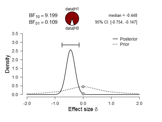
### generate data ###
set.seed(1)
x <- rnorm(30, 0.15)
### calculate Bayes factor ###
library(BayesFactor)
BF <- extractBF(ttestBF(x, rscale = "medium"), onlybf = TRUE)
### plot ###
.plotPosterior.ttest(x = x, rscale = "medium", BF = BF)
#monte carlo t test simulation


#install.packages("MonteCarlo")
library(MonteCarlo)


# Define function that generates data and applies the method of interest

ttest<-function(n,loc,scale){

  # generate sample:
    sample<-rnorm(n, loc, scale)

  # calculate test statistic:
    stat<-sqrt(n)*mean(sample)/sd(sample)

  # get test decision:
    decision<-abs(stat)>1.96

  # return result:
    return(list("decision"=decision))
}

# define parameter grid:

  n_grid<-c(50,100,250,500)
  loc_grid<-seq(0,1,0.2)
  scale_grid<-c(1,2)

# collect parameter grids in list:
  param_list=list("n"=n_grid, "loc"=loc_grid, "scale"=scale_grid)

# run simulation:

  MC_result<-MonteCarlo(func=ttest, nrep=1000, param_list=param_list)

  summary(MC_result)
#install.packages("RWordPress", repos="http://www.omegahat.org/R", build=TRUE)
library(RWordPress)
options(WordPressLogin=c(user="password"),
        WordPressURL="http://your_wp_installation.org/xmlrpc.php")
#[code lang='r']
#...
#[/code]
knit_hooks$set(output=function(x, options) paste("\\[code\\]\n", x, "\\[/code\\]\n", sep=""))
knit_hooks$set(source=function(x, options) paste("\\[code lang='r'\\]\n", x, "\\[/code\\]\n", sep=""))

knit2wp <- function(file) {
    require(XML)
    content <- readLines(file)
    content <- htmlTreeParse(content, trim=FALSE)

    ## WP will add the h1 header later based on the title, so delete here
    content$children$html$children$body$children$h1 <- NULL
    content <- paste(capture.output(print(content$children$html$children$body,
                                          indent=FALSE, tagSeparator="")),
                     collapse="\n")
    content <- gsub("<?.body>", "", content)         # remove body tag

    ## enclose code snippets in SyntaxHighlighter format
    content <- gsub("<?pre><code class=\"r\">", "\\[code lang='r'\\]\\\n",
                    content)
    content <- gsub("<?pre><code class=\"no-highlight\">", "\\[code\\]\\\n",
                    content)
    content <- gsub("<?pre><code>", "\\[code\\]\\\n", content)
    content <- gsub("<?/code></pre>", "\\[/code\\]\\\n", content)
    return(content)
}

newPost(content=list(description=knit2wp('rerWorkflow.html'),
                     title='Workflow: Post R markdown to WordPress',
                     categories=c('R')),
        publish=FALSE)

postID <- 99                    # post id returned by newPost()
editPost(postID,
         content=list(description=knit2wp('rerWorkflow.html'),
                      title='Workflow: Post R markdown to WordPress',
                      categories=c('R')),
         publish=FALSE)