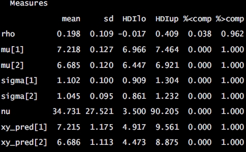
Numerical summary for all parameters associated with experimental condition V01 and V11 and their corresponding 95% posterior high density credible intervals.

• ρ (rho): The correlation between experimental condition V00 and V10
• μ1 (mu[1]): The mean of V00
• σ1 (sigma[1]): The scale of V00, a consistent estimate of SD when nu is large.
• μ2 (mu[2]): the mean of V10
• σ1 (sigma[2]): the scale of V10
• ν (nu): The degrees-of-freedom for the bivariate t distribution
• xy_pred[1]: The posterior predictive distribution of V00
• xy_pred[2]: The posterior predictive distribution of V10

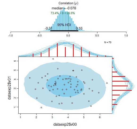
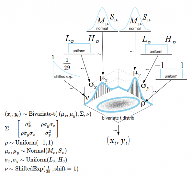
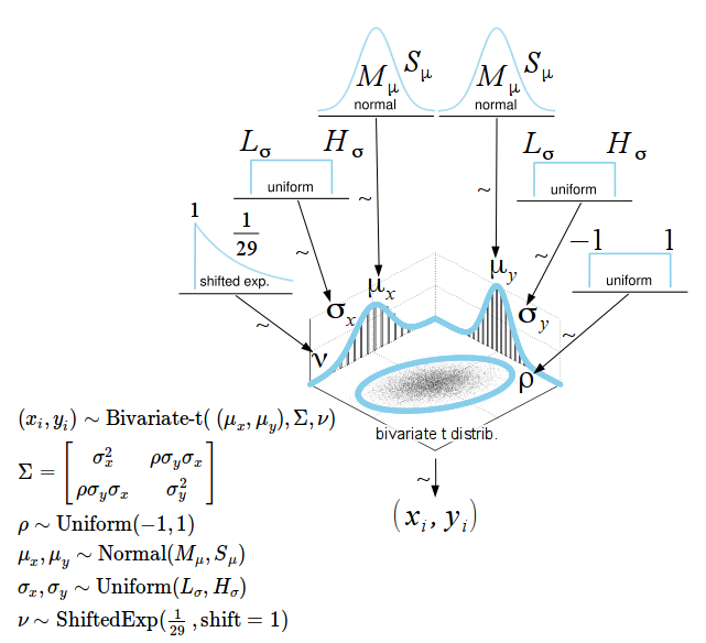
Visualisation of the results of the Bayesian correlational analysis for experimental condition V00 and V01 with associated posterior high density credible intervals and marginal posterior predictive plots.

The upper panel of the plot displays the posterior distribution for the correlation ρ (rho) with its associated 95% HDI. In addition, the lower panel of the plot shows the original empirical data with superimposed posterior predictive distributions. The posteriors predictive distributions allow to predict new data and can also be utilised to assess the model fit. It can be seen that the model fits the data reasonably well. The two histograms (in red) visualise the marginal distributions of the experimental data. The dark-blue ellipse encompasses the 50% highest density region and the light-blue ellipse spans the 95% high density region, thereby providing intuitive visual insights into the probabilistic distribution of the data (Hollowood, 2016). The Bayesian analysis provides much more detailed and precise information compared to the classical frequentist Pearsonian approach.

JAGS model code for the correlational analysis

# Model code for the Bayesian alternative to Pearson's correlation test.
# (Bååth, 2014)
require(rjags)
#(Plummer, 2016)
#download data from webserver and import as table
Dataexp2 <-
read.table("http://www.irrational-decisions.com/phd-thesis/dataexp2.csv", header=TRUE, sep=",", na.strings="NA", dec=".", strip.white=TRUE)
# Setting up the data
x <- dataexp1$v01
y <- dataexp1$v11
xy <- cbind(x, y)
# The model string written in the JAGS language
model_string <- "model {
for(i in 1:n) {
xy[i,1:2] ~ dmt(mu[], prec[ , ], nu)
}
xy_pred[1:2] ~ dmt(mu[], prec[ , ], nu)
# JAGS parameterizes the multivariate t using precision (inverse of variance)
# rather than variance, therefore here inverting the covariance matrix.
prec[1:2,1:2] <- inverse(cov[,])
# Constructing the covariance matrix
cov[1,1] <- sigma[1] * sigma[1]
cov[1,2] <- sigma[1] * sigma[2] * rho
cov[2,1] <- sigma[1] * sigma[2] * rho
cov[2,2] <- sigma[2] * sigma[2]
# Priors
rho ~ dunif(-1, 1)
sigma[1] ~ dunif(sigmaLow, sigmaHigh)
sigma[2] ~ dunif(sigmaLow, sigmaHigh)
mu[1] ~ dnorm(mean_mu, precision_mu)
mu[2] ~ dnorm(mean_mu, precision_mu)
nu <- nuMinusOne+1
nuMinusOne ~ dexp(1/29)
}"
# Initializing the data list and setting parameters for the priors
# that in practice will result in flat priors on mu and sigma.
data_list = list(
xy = xy,
n = length(x),
mean_mu = mean(c(x, y), trim=0.2) ,
precision_mu = 1 / (max(mad(x), mad(y))^2 * 1000000),
sigmaLow = min(mad(x), mad(y)) / 1000 ,
sigmaHigh = max(mad(x), mad(y)) * 1000)
# Initializing parameters to sensible starting values helps the convergence
# of the MCMC sampling. Here using robust estimates of the mean (trimmed)
# and standard deviation (MAD).
inits_list = list(mu=c(mean(x, trim=0.2), mean(y, trim=0.2)), rho=cor(x, y, method="spearman"),
sigma = c(mad(x), mad(y)), nuMinusOne = 5)
# The parameters to monitor.
params <- c("rho", "mu", "sigma", "nu", "xy_pred")
# Running the model
model <- jags.model(textConnection(model_string), data = data_list,
inits = inits_list, n.chains = 3, n.adapt=1000)
update(model, 500)
samples <- coda.samples(model, params, n.iter=5000)
# Inspecting the posterior
plot(samples)
summary(samples)

Pertinent references