The Bayesian inferential approach provides rich information about the estimated distribution of several parameters of interest, i.e., it provides the distribution of the estimates of μ and σ of both experimental conditions and the associated effect sizes. Specifically, the method provides the “relative credibility” of all possible differences between means, standard deviations (Kruschke, 2013). Inferential conclusions about null hypotheses can be drawn based on these credibility values. In contrast to conventional NHST, uninformative (and frequently misleading124) p values are redundant in the Bayesian framework. Moreover, the Bayesian parameter estimation approach enables the researcher to accept null hypotheses. NHST, on the other, only allows the researcher to reject such null hypotheses. The critical reader might object why one would use complex Bayesian computations for the relatively simple within-group design at hand. One might argue that a more parsimonious analytic approach is preferable. Exactly this question has been articulated before in a paper entitled “Bayesian computation: a statistical revolution” which was published in the Philosophical Transactions of the Royal Society: “Thus, if your primary question of interest can be simply expressed in a form amenable to a t test, say, there really is no need to try and apply the full Bayesian machinery to so simple a problem” (S. P. Brooks, 2003, p. 2694). The answer is straightforward: “Decisions based on Bayesian parameter estimation are better founded than those based on NHST, whether the decisions derived by the two methods agree or not. The conclusion is bold but simple: Bayesian parameter estimation supersedes the NHST t test” (Kruschke, 2013, p. 573).
Bayesian parameter estimation is more informative than NHST125 (independent of the complexity of the research question under investigation). Moreover, the conclusions drawn from Bayesian parameter estimates do not necessarily converge with those based on NHST. This has been empirically demonstrated beyond doubt by several independent researchers (Kruschke, 2013; Rouder et al., 2009).
The function ‘BEST.R’ can be downloaded from the CRAN (Comprehensive R Archive Network) repository under the following URL:
https://cran.r-project.org/web/packages/BEST/index.html
The BEST function has been ported to MATLAB and Python.
Matlab version of BEST: https://github.com/NilsWinter/matlab-bayesian-estimation/
Python version of BEST: https://github.com/strawlab/best/
# MODIFIED 2015 DEC 02.
# John K. Kruschke
# johnkruschke@gmail.com
# http://www.indiana.edu/~kruschke/BEST/
#
# This program is believed to be free of errors, but it comes with no guarantee!
# The user bears all responsibility for interpreting the results.
# Please check the webpage above for updates or corrections.
#
### ***************************************************************
### ******** SEE FILE BESTexample.R FOR INSTRUCTIONS **************
### ***************************************************************

# Load various essential functions:
source("DBDA2E-utilities.R")

BESTmcmc = function( y1 , y2 ,
                     priorOnly=FALSE , showMCMC=FALSE ,
                     numSavedSteps=20000 , thinSteps=1 ,
                     mu1PriorMean = mean(c(y1,y2)) ,
                     mu1PriorSD = sd(c(y1,y2))*5 ,
                     mu2PriorMean = mean(c(y1,y2)) ,
                     mu2PriorSD = sd(c(y1,y2))*5 ,
                     sigma1PriorMode = sd(c(y1,y2)) ,
                     sigma1PriorSD = sd(c(y1,y2))*5 ,
                     sigma2PriorMode = sd(c(y1,y2)) ,
                     sigma2PriorSD = sd(c(y1,y2))*5 ,
                     nuPriorMean = 30 ,
                     nuPriorSD = 30 ,
                     runjagsMethod=runjagsMethodDefault ,
                     nChains=nChainsDefault ) {
  # This function generates an MCMC sample from the posterior distribution.
  # Description of arguments:
  # showMCMC is a flag for displaying diagnostic graphs of the chains.
  #    If F (the default), no chain graphs are displayed. If T, they are.

  #------------------------------------------------------------------------------
  # THE DATA.
  # Load the data:
  y = c( y1 , y2 ) # combine data into one vector
  x = c( rep(1,length(y1)) , rep(2,length(y2)) ) # create group membership code
  Ntotal = length(y)
  # Specify the data and prior constants in a list, for later shipment to JAGS:
  if ( priorOnly ) {
    dataList = list(
      #  y = y ,
      x = x ,
      Ntotal = Ntotal ,
      mu1PriorMean = mu1PriorMean ,
      mu1PriorSD = mu1PriorSD ,
      mu2PriorMean = mu2PriorMean ,
      mu2PriorSD = mu2PriorSD ,
      Sh1 = gammaShRaFromModeSD( mode=sigma1PriorMode ,
                                 sd=sigma1PriorSD )$shape ,
      Ra1 = gammaShRaFromModeSD( mode=sigma1PriorMode ,
                                 sd=sigma1PriorSD )$rate ,
      Sh2 = gammaShRaFromModeSD( mode=sigma2PriorMode ,
                                 sd=sigma2PriorSD )$shape ,
      Ra2 = gammaShRaFromModeSD( mode=sigma2PriorMode ,
                                 sd=sigma2PriorSD )$rate ,
      ShNu = gammaShRaFromMeanSD( mean=nuPriorMean , sd=nuPriorSD )$shape ,
      RaNu = gammaShRaFromMeanSD( mean=nuPriorMean , sd=nuPriorSD )$rate
    )
  } else {
    dataList = list(
      y = y ,
      x = x ,
      Ntotal = Ntotal ,
      mu1PriorMean = mu1PriorMean ,
      mu1PriorSD = mu1PriorSD ,
      mu2PriorMean = mu2PriorMean ,
      mu2PriorSD = mu2PriorSD ,
      Sh1 = gammaShRaFromModeSD( mode=sigma1PriorMode ,
                                 sd=sigma1PriorSD )$shape ,
      Ra1 = gammaShRaFromModeSD( mode=sigma1PriorMode ,
                                 sd=sigma1PriorSD )$rate ,
      Sh2 = gammaShRaFromModeSD( mode=sigma2PriorMode ,
                                 sd=sigma2PriorSD )$shape ,
      Ra2 = gammaShRaFromModeSD( mode=sigma2PriorMode ,
                                 sd=sigma2PriorSD )$rate ,
      ShNu = gammaShRaFromMeanSD( mean=nuPriorMean , sd=nuPriorSD )$shape ,
      RaNu = gammaShRaFromMeanSD( mean=nuPriorMean , sd=nuPriorSD )$rate
    )
  }

  #----------------------------------------------------------------------------
  # THE MODEL.
  modelString = "
  model {
    for ( i in 1:Ntotal ) {
      y[i] ~ dt( mu[x[i]] , 1/sigma[x[i]]^2 , nu )
    }
    mu[1] ~ dnorm( mu1PriorMean , 1/mu1PriorSD^2 )  # prior for mu[1]
    sigma[1] ~ dgamma( Sh1 , Ra1 )     # prior for sigma[1]
    mu[2] ~ dnorm( mu2PriorMean , 1/mu2PriorSD^2 )  # prior for mu[2]
    sigma[2] ~ dgamma( Sh2 , Ra2 )     # prior for sigma[2]
    nu ~ dgamma( ShNu , RaNu ) # prior for nu
  }
  " # close quote for modelString
  # Write out modelString to a text file
  writeLines( modelString , con="BESTmodel.txt" )

  #------------------------------------------------------------------------------
  # INTIALIZE THE CHAINS.
  # Initial values of MCMC chains based on data:
  mu = c( mean(y1) , mean(y2) )
  sigma = c( sd(y1) , sd(y2) )
  # Regarding initial values in next line: (1) sigma will tend to be too big if
  # the data have outliers, and (2) nu starts at 5 as a moderate value. These
  # initial values keep the burn-in period moderate.
  initsList = list( mu = mu , sigma = sigma , nu = 5 )

  #------------------------------------------------------------------------------
  # RUN THE CHAINS

  parameters = c( "mu" , "sigma" , "nu" )     # The parameters to be monitored
  adaptSteps = 500               # Number of steps to "tune" the samplers
  burnInSteps = 1000

  runJagsOut <- run.jags( method=runjagsMethod ,
                          model="BESTmodel.txt" ,
                          monitor=parameters ,
                          data=dataList ,
                          inits=initsList ,
                          n.chains=nChains ,
                          adapt=adaptSteps ,
                          burnin=burnInSteps ,
                          sample=ceiling(numSavedSteps/nChains) ,
                          thin=thinSteps ,
                          summarise=FALSE ,
                          plots=FALSE )
  codaSamples = as.mcmc.list( runJagsOut )
  # resulting codaSamples object has these indices:
  #   codaSamples[[ chainIdx ]][ stepIdx , paramIdx ]

  ## Original version, using rjags:
  #   nChains = 3
  #   nIter = ceiling( ( numSavedSteps * thinSteps ) / nChains )
  #   # Create, initialize, and adapt the model:
  #   jagsModel = jags.model( "BESTmodel.txt" , data=dataList , inits=initsList ,
  #                           n.chains=nChains , n.adapt=adaptSteps )
  #   # Burn-in:
  #   cat( "Burning in the MCMC chain...\n" )
  #   update( jagsModel , n.iter=burnInSteps )
  #   # The saved MCMC chain:
  #   cat( "Sampling final MCMC chain...\n" )
  #   codaSamples = coda.samples( jagsModel , variable.names=parameters ,
  #                               n.iter=nIter , thin=thinSteps )

  #------------------------------------------------------------------------------
  # EXAMINE THE RESULTS
  if ( showMCMC ) {
    for ( paramName in varnames(codaSamples) ) {
      diagMCMC( codaSamples , parName=paramName )
    }
  }

  # Convert coda-object codaSamples to matrix object for easier handling.
  # But note that this concatenates the different chains into one long chain.
  # Result is mcmcChain[ stepIdx , paramIdx ]
  mcmcChain = as.matrix( codaSamples )
  return( mcmcChain )

} # end function BESTmcmc

#==============================================================================

BESTsummary = function( y1 , y2 , mcmcChain ) {
  #source("HDIofMCMC.R") # in DBDA2E-utilities.R
  mcmcSummary = function( paramSampleVec , compVal=NULL ) {
    meanParam = mean( paramSampleVec )
    medianParam = median( paramSampleVec )
    dres = density( paramSampleVec )
    modeParam = dres$x[which.max(dres$y)]
    hdiLim = HDIofMCMC( paramSampleVec )
    if ( !is.null(compVal) ) {
      pcgtCompVal = ( 100 * sum( paramSampleVec > compVal )
                      / length( paramSampleVec ) )
    } else {
      pcgtCompVal=NA
    }
    return( c( meanParam , medianParam , modeParam , hdiLim , pcgtCompVal ) )
  }
  # Define matrix for storing summary info:
  summaryInfo = matrix( 0 , nrow=9 , ncol=6 , dimnames=list(
    PARAMETER=c( "mu1" , "mu2" , "muDiff" , "sigma1" , "sigma2" , "sigmaDiff" ,
                 "nu" , "nuLog10" , "effSz" ),
    SUMMARY.INFO=c( "mean" , "median" , "mode" , "HDIlow" , "HDIhigh" ,
                    "pcgtZero" )
  ) )
  summaryInfo[ "mu1" , ] = mcmcSummary( mcmcChain[,"mu[1]"] )
  summaryInfo[ "mu2" , ] = mcmcSummary( mcmcChain[,"mu[2]"] )
  summaryInfo[ "muDiff" , ] = mcmcSummary( mcmcChain[,"mu[1]"]
                                           - mcmcChain[,"mu[2]"] ,
                                           compVal=0 )
  summaryInfo[ "sigma1" , ] = mcmcSummary( mcmcChain[,"sigma[1]"] )
  summaryInfo[ "sigma2" , ] = mcmcSummary( mcmcChain[,"sigma[2]"] )
  summaryInfo[ "sigmaDiff" , ] = mcmcSummary( mcmcChain[,"sigma[1]"]
                                              - mcmcChain[,"sigma[2]"] ,
                                              compVal=0 )
  summaryInfo[ "nu" , ] = mcmcSummary( mcmcChain[,"nu"] )
  summaryInfo[ "nuLog10" , ] = mcmcSummary( log10(mcmcChain[,"nu"]) )

  N1 = length(y1)
  N2 = length(y2)
  effSzChain = ( ( mcmcChain[,"mu[1]"] - mcmcChain[,"mu[2]"] )
                 / sqrt( ( mcmcChain[,"sigma[1]"]^2
                           + mcmcChain[,"sigma[2]"]^2 ) / 2 ) )
  summaryInfo[ "effSz" , ] = mcmcSummary( effSzChain , compVal=0 )
  # Or, use sample-size weighted version:
  # effSz = ( mu1 - mu2 ) / sqrt( ( sigma1^2 *(N1-1) + sigma2^2 *(N2-1) )
  #                               / (N1+N2-2) )
  # Be sure also to change plot label in BESTplot function, below.
  return( summaryInfo )
}

#==============================================================================

BESTplot = function( y1 , y2 , mcmcChain , ROPEm=NULL , ROPEsd=NULL ,
                     ROPEeff=NULL , showCurve=FALSE , pairsPlot=FALSE ) {
  # This function plots the posterior distribution (and data).
  # Description of arguments:
  # y1 and y2 are the data vectors.
  # mcmcChain is a list of the type returned by function BTT.
  # ROPEm is a two element vector, such as c(-1,1), specifying the limit
  #   of the ROPE on the difference of means.
  # ROPEsd is a two element vector, such as c(-1,1), specifying the limit
  #   of the ROPE on the difference of standard deviations.
  # ROPEeff is a two element vector, such as c(-1,1), specifying the limit
  #   of the ROPE on the effect size.
  # showCurve is TRUE or FALSE and indicates whether the posterior should
  #   be displayed as a histogram (by default) or by an approximate curve.
  # pairsPlot is TRUE or FALSE and indicates whether scatterplots of pairs
  #   of parameters should be displayed.
  mu1 = mcmcChain[,"mu[1]"]
  mu2 = mcmcChain[,"mu[2]"]
  sigma1 = mcmcChain[,"sigma[1]"]
  sigma2 = mcmcChain[,"sigma[2]"]
  nu = mcmcChain[,"nu"]
  if ( pairsPlot ) {
    # Plot the parameters pairwise, to see correlations:
    openGraph(width=7,height=7)
    nPtToPlot = 1000
    plotIdx = floor(seq(1,length(mu1),by=length(mu1)/nPtToPlot))
    panel.cor = function(x, y, digits=2, prefix="", cex.cor, ...) {
      usr = par("usr"); on.exit(par(usr))
      par(usr = c(0, 1, 0, 1))
      r = (cor(x, y))
      txt = format(c(r, 0.123456789), digits=digits)[1]
      txt = paste(prefix, txt, sep="")
      if(missing(cex.cor)) cex.cor <- 0.8/strwidth(txt)
      text(0.5, 0.5, txt, cex=1.25 ) # was cex=cex.cor*r
    }
    pairs( cbind( mu1 , mu2 , sigma1 , sigma2 , log10(nu) )[plotIdx,] ,
           labels=c( expression(mu[1]) , expression(mu[2]) ,
                     expression(sigma[1]) , expression(sigma[2]) ,
                     expression(log10(nu)) ) ,
           lower.panel=panel.cor , col="skyblue" )
  }
  # source("plotPost.R") # in DBDA2E-utilities.R
  # Set up window and layout:
  openGraph(width=6.0,height=8.0)
  layout( matrix( c(4,5,7,8,3,1,2,6,9,10) , nrow=5, byrow=FALSE ) )
  par( mar=c(3.5,3.5,2.5,0.5) , mgp=c(2.25,0.7,0) )

  # Select thinned steps in chain for plotting of posterior predictive curves:
  chainLength = NROW( mcmcChain )
  nCurvesToPlot = 30
  stepIdxVec = seq( 1 , chainLength , floor(chainLength/nCurvesToPlot) )
  xRange = range( c(y1,y2) )
  if ( isTRUE( all.equal( xRange[2] , xRange[1] ) ) ) {
    meanSigma = mean( c(sigma1,sigma2) )
    xRange = xRange + c( -meanSigma , meanSigma )
  }
  xLim = c( xRange[1]-0.1*(xRange[2]-xRange[1]) ,
            xRange[2]+0.1*(xRange[2]-xRange[1]) )
  xVec = seq( xLim[1] , xLim[2] , length=200 )
  maxY = max( dt( 0 , df=max(nu[stepIdxVec]) ) /
                min(c(sigma1[stepIdxVec],sigma2[stepIdxVec])) )
  # Plot data y1 and smattering of posterior predictive curves:
  stepIdx = 1
  plot( xVec , dt( (xVec-mu1[stepIdxVec[stepIdx]])/sigma1[stepIdxVec[stepIdx]] ,
                   df=nu[stepIdxVec[stepIdx]] )/sigma1[stepIdxVec[stepIdx]] ,
        ylim=c(0,maxY) , cex.lab=1.75 ,
        type="l" , col="skyblue" , lwd=1 , xlab="y" , ylab="p(y)" ,
        main="Data Group 1 w. Post. Pred." )
  for ( stepIdx in 2:length(stepIdxVec) ) {
    lines(xVec, dt( (xVec-mu1[stepIdxVec[stepIdx]])/sigma1[stepIdxVec[stepIdx]] ,
                    df=nu[stepIdxVec[stepIdx]] )/sigma1[stepIdxVec[stepIdx]] ,
          type="l" , col="skyblue" , lwd=1 )
  }
  histBinWd = median(sigma1)/2
  histCenter = mean(mu1)
  histBreaks = sort( c( seq( histCenter-histBinWd/2 , min(xVec)-histBinWd/2 ,
                             -histBinWd ),
                        seq( histCenter+histBinWd/2 , max(xVec)+histBinWd/2 ,
                             histBinWd ) , xLim ) )
  histInfo = hist( y1 , plot=FALSE , breaks=histBreaks )
  yPlotVec = histInfo$density
  yPlotVec[ yPlotVec==0.0 ] = NA
  xPlotVec = histInfo$mids
  xPlotVec[ yPlotVec==0.0 ] = NA
  points( xPlotVec , yPlotVec , type="h" , lwd=3 , col="red" )
  text( max(xVec) , maxY , bquote(N[1]==.(length(y1))) , adj=c(1.1,1.1) )
  # Plot data y2 and smattering of posterior predictive curves:
  stepIdx = 1
  plot( xVec , dt( (xVec-mu2[stepIdxVec[stepIdx]])/sigma2[stepIdxVec[stepIdx]] ,
                   df=nu[stepIdxVec[stepIdx]] )/sigma2[stepIdxVec[stepIdx]] ,
        ylim=c(0,maxY) , cex.lab=1.75 ,
        type="l" , col="skyblue" , lwd=1 , xlab="y" , ylab="p(y)" ,
        main="Data Group 2 w. Post. Pred." )
  for ( stepIdx in 2:length(stepIdxVec) ) {
    lines(xVec, dt( (xVec-mu2[stepIdxVec[stepIdx]])/sigma2[stepIdxVec[stepIdx]] ,
                    df=nu[stepIdxVec[stepIdx]] )/sigma2[stepIdxVec[stepIdx]] ,
          type="l" , col="skyblue" , lwd=1 )
  }
  histBinWd = median(sigma2)/2
  histCenter = mean(mu2)
  histBreaks = sort( c( seq( histCenter-histBinWd/2 , min(xVec)-histBinWd/2 ,
                             -histBinWd ),
                        seq( histCenter+histBinWd/2 , max(xVec)+histBinWd/2 ,
                             histBinWd ) , xLim ) )
  histInfo = hist( y2 , plot=FALSE , breaks=histBreaks )
  yPlotVec = histInfo$density
  yPlotVec[ yPlotVec==0.0 ] = NA
  xPlotVec = histInfo$mids
  xPlotVec[ yPlotVec==0.0 ] = NA
  points( xPlotVec , yPlotVec , type="h" , lwd=3 , col="red" )
  text( max(xVec) , maxY , bquote(N[2]==.(length(y2))) , adj=c(1.1,1.1) )

  # Plot posterior distribution of parameter nu:
  histInfo = plotPost( log10(nu) , col="skyblue" , # breaks=30 ,
                       showCurve=showCurve ,
                       xlab=bquote("log10("*nu*")") , cex.lab = 1.75 ,
                       cenTend=c("mode","median","mean")[1] ,
                       main="Normality" ) #  (<0.7 suggests kurtosis)

  # Plot posterior distribution of parameters mu1, mu2, and their difference:
  xlim = range( c( mu1 , mu2 ) )
  histInfo = plotPost( mu1 ,  xlim=xlim , cex.lab = 1.75 ,
                       showCurve=showCurve ,
                       xlab=bquote(mu[1]) , main=paste("Group",1,"Mean") ,
                       col="skyblue" )
  histInfo = plotPost( mu2 ,  xlim=xlim , cex.lab = 1.75 ,
                       showCurve=showCurve ,
                       xlab=bquote(mu[2]) , main=paste("Group",2,"Mean") ,
                       col="skyblue" )
  histInfo = plotPost( mu1-mu2 , compVal=0 ,  showCurve=showCurve ,
                       xlab=bquote(mu[1] - mu[2]) , cex.lab = 1.75 , ROPE=ROPEm ,
                       main="Difference of Means" , col="skyblue" )

  # Plot posterior distribution of param's sigma1, sigma2, and their difference:
  xlim=range( c( sigma1 , sigma2 ) )
  histInfo = plotPost( sigma1 ,  xlim=xlim , cex.lab = 1.75 ,
                       showCurve=showCurve ,
                       xlab=bquote(sigma[1]) , main=paste("Group",1,"Std. Dev.") ,
                       col="skyblue" , cenTend=c("mode","median","mean")[1] )
  histInfo = plotPost( sigma2 ,  xlim=xlim , cex.lab = 1.75 ,
                       showCurve=showCurve ,
                       xlab=bquote(sigma[2]) , main=paste("Group",2,"Std. Dev.") ,
                       col="skyblue" , cenTend=c("mode","median","mean")[1] )
  histInfo = plotPost( sigma1-sigma2 ,
                       compVal=0 ,  showCurve=showCurve ,
                       xlab=bquote(sigma[1] - sigma[2]) , cex.lab = 1.75 ,
                       ROPE=ROPEsd ,
                       main="Difference of Std. Dev.s" , col="skyblue" ,
                       cenTend=c("mode","median","mean")[1] )

  # Plot of estimated effect size. Effect size is d-sub-a from
  # Macmillan & Creelman, 1991; Simpson & Fitter, 1973; Swets, 1986a, 1986b.
  effectSize = ( mu1 - mu2 ) / sqrt( ( sigma1^2 + sigma2^2 ) / 2 )
  histInfo = plotPost( effectSize , compVal=0 ,  ROPE=ROPEeff ,
                       showCurve=showCurve ,
                       xlab=bquote( (mu[1]-mu[2])
                                    /sqrt((sigma[1]^2 +sigma[2]^2 )/2 ) ),
                       cenTend=c("mode","median","mean")[1] , cex.lab=1.0 , main="Effect Size" ,
                       col="skyblue" )
  # Or use sample-size weighted version:
  # Hedges 1981; Wetzels, Raaijmakers, Jakab & Wagenmakers 2009.
  # N1 = length(y1)
  # N2 = length(y2)
  # effectSize = ( mu1 - mu2 ) / sqrt( ( sigma1^2 *(N1-1) + sigma2^2 *(N2-1) )
  #                                    / (N1+N2-2) )
  # Be sure also to change BESTsummary function, above.
  # histInfo = plotPost( effectSize , compVal=0 ,  ROPE=ROPEeff ,
  #          showCurve=showCurve ,
  #          xlab=bquote( (mu[1]-mu[2])
  #          /sqrt((sigma[1]^2 *(N[1]-1)+sigma[2]^2 *(N[2]-1))/(N[1]+N[2]-2)) ),
  #          cenTend=c("mode","median","mean")[1] , cex.lab=1.0 , main="Effect Size" , col="skyblue" )
  return( BESTsummary( y1 , y2 , mcmcChain ) )
} # end of function BESTplot

#==============================================================================

BESTpower = function( mcmcChain , N1 , N2 , ROPEm , ROPEsd , ROPEeff ,
                      maxHDIWm , maxHDIWsd , maxHDIWeff , nRep=200 ,
                      mcmcLength=10000 , saveName="BESTpower.Rdata" ,
                      showFirstNrep=0 ) {
  # This function estimates power.
  # Description of arguments:
  # mcmcChain is a matrix of the type returned by function BESTmcmc.
  # N1 and N2 are sample sizes for the two groups.
  # ROPEm is a two element vector, such as c(-1,1), specifying the limit
  #   of the ROPE on the difference of means.
  # ROPEsd is a two element vector, such as c(-1,1), specifying the limit
  #   of the ROPE on the difference of standard deviations.
  # ROPEeff is a two element vector, such as c(-1,1), specifying the limit
  #   of the ROPE on the effect size.
  # maxHDIWm is the maximum desired width of the 95% HDI on the difference
  #   of means.
  # maxHDIWsd is the maximum desired width of the 95% HDI on the difference
  #   of standard deviations.
  # maxHDIWeff is the maximum desired width of the 95% HDI on the effect size.
  # nRep is the number of simulated experiments used to estimate the power.
  #source("HDIofMCMC.R") # in DBDA2E-utilities.R
  #source("HDIofICDF.R") # in DBDA2E-utilities.R
  chainLength = NROW( mcmcChain )
  # Select thinned steps in chain for posterior predictions:
  stepIdxVec = seq( 1 , chainLength , floor(chainLength/nRep) )
  goalTally = list( HDIm.gt.ROPE = c(0) ,
                    HDIm.lt.ROPE = c(0) ,
                    HDIm.in.ROPE = c(0) ,
                    HDIm.wd.max = c(0) ,
                    HDIsd.gt.ROPE = c(0) ,
                    HDIsd.lt.ROPE = c(0) ,
                    HDIsd.in.ROPE = c(0) ,
                    HDIsd.wd.max = c(0) ,
                    HDIeff.gt.ROPE = c(0) ,
                    HDIeff.lt.ROPE = c(0) ,
                    HDIeff.in.ROPE = c(0) ,
                    HDIeff.wd.max = c(0) )
  power     = list( HDIm.gt.ROPE = c(0,0,0) ,
                    HDIm.lt.ROPE = c(0,0,0) ,
                    HDIm.in.ROPE = c(0,0,0) ,
                    HDIm.wd.max = c(0,0,0) ,
                    HDIsd.gt.ROPE = c(0,0,0) ,
                    HDIsd.lt.ROPE = c(0,0,0) ,
                    HDIsd.in.ROPE = c(0,0,0) ,
                    HDIsd.wd.max = c(0,0,0) ,
                    HDIeff.gt.ROPE = c(0,0,0) ,
                    HDIeff.lt.ROPE = c(0,0,0) ,
                    HDIeff.in.ROPE = c(0,0,0) ,
                    HDIeff.wd.max = c(0,0,0) )
  nSim = 0
  for ( stepIdx in stepIdxVec ) {
    nSim = nSim + 1
    cat( "\n:::::::::::::::::::::::::::::::::::::::::::::::::::::::::::::::\n" )
    cat( paste( "Power computation: Simulated Experiment" , nSim , "of" ,
                length(stepIdxVec) , ":\n\n" ) )
    # Get parameter values for this simulation:
    mu1Val = mcmcChain[stepIdx,"mu[1]"]
    mu2Val = mcmcChain[stepIdx,"mu[2]"]
    sigma1Val = mcmcChain[stepIdx,"sigma[1]"]
    sigma2Val = mcmcChain[stepIdx,"sigma[2]"]
    nuVal = mcmcChain[stepIdx,"nu"]
    # Generate simulated data:
    y1 = rt( N1 , df=nuVal ) * sigma1Val + mu1Val
    y2 = rt( N2 , df=nuVal ) * sigma2Val + mu2Val
    # Get posterior for simulated data:
    simChain = BESTmcmc( y1, y2, numSavedSteps=mcmcLength, thinSteps=1,
                         showMCMC=FALSE )
    if (nSim <= showFirstNrep ) {
      BESTplot( y1, y2, simChain, ROPEm=ROPEm, ROPEsd=ROPEsd, ROPEeff=ROPEeff )
    }
    # Assess which goals were achieved and tally them:
    HDIm = HDIofMCMC( simChain[,"mu[1]"] - simChain[,"mu[2]"] )
    if ( HDIm[1] > ROPEm[2] ) {
      goalTally$HDIm.gt.ROPE = goalTally$HDIm.gt.ROPE + 1 }
    if ( HDIm[2] < ROPEm[1] ) {
      goalTally$HDIm.lt.ROPE = goalTally$HDIm.lt.ROPE + 1 }
    if ( HDIm[1] > ROPEm[1] &  HDIm[2] < ROPEm[2] ) {
      goalTally$HDIm.in.ROPE = goalTally$HDIm.in.ROPE + 1 }
    if ( HDIm[2] - HDIm[1] < maxHDIWm ) {
      goalTally$HDIm.wd.max = goalTally$HDIm.wd.max + 1 }
    HDIsd = HDIofMCMC( simChain[,"sigma[1]"] - simChain[,"sigma[2]"] )
    if ( HDIsd[1] > ROPEsd[2] ) {
      goalTally$HDIsd.gt.ROPE = goalTally$HDIsd.gt.ROPE + 1 }
    if ( HDIsd[2] < ROPEsd[1] ) {
      goalTally$HDIsd.lt.ROPE = goalTally$HDIsd.lt.ROPE + 1 }
    if ( HDIsd[1] > ROPEsd[1] &  HDIsd[2] < ROPEsd[2] ) {
      goalTally$HDIsd.in.ROPE = goalTally$HDIsd.in.ROPE + 1 }
    if ( HDIsd[2] - HDIsd[1] < maxHDIWsd ) {
      goalTally$HDIsd.wd.max = goalTally$HDIsd.wd.max + 1 }

    HDIeff = HDIofMCMC( ( simChain[,"mu[1]"] - simChain[,"mu[2]"] ) /
                          sqrt( ( simChain[,"sigma[1]"]^2 + simChain[,"sigma[2]"]^2 ) / 2 ) )
    if ( HDIeff[1] > ROPEeff[2] ) {
      goalTally$HDIeff.gt.ROPE = goalTally$HDIeff.gt.ROPE + 1 }
    if ( HDIeff[2] < ROPEeff[1] ) {
      goalTally$HDIeff.lt.ROPE = goalTally$HDIeff.lt.ROPE + 1 }
    if ( HDIeff[1] > ROPEeff[1] &  HDIeff[2] < ROPEeff[2] ) {
      goalTally$HDIeff.in.ROPE = goalTally$HDIeff.in.ROPE + 1 }
    if ( HDIeff[2] - HDIeff[1] < maxHDIWeff ) {
      goalTally$HDIeff.wd.max = goalTally$HDIeff.wd.max + 1 }

    for ( i in 1:length(goalTally) ) {
      s1 = 1 + goalTally[[i]]
      s2 = 1 + ( nSim - goalTally[[i]] )
      power[[i]][1] = s1/(s1+s2)
      power[[i]][2:3] = HDIofICDF( qbeta , shape1=s1 , shape2=s2 )
    }
    cat( "\nAfter ", nSim ,
         " Simulated Experiments, Power Is: \n( mean, HDI_low, HDI_high )\n" )
    for ( i in 1:length(power) ) {
      cat( names(power[i]) , round(power[[i]],3) , "\n" )
    }
    save( nSim , power , file=saveName )
  }
  return( power )
} # end of function BESTpower

#==============================================================================

makeData = function( mu1 , sd1 , mu2 , sd2 , nPerGrp ,
                     pcntOut=0 , sdOutMult=2.0 , rnd.seed=NULL ) {
  # Auxilliary function for generating random values from a
  # mixture of normal distibutions.
  if(!is.null(rnd.seed)){set.seed(rnd.seed)} # Set seed for random values.
  nOut = ceiling(nPerGrp*pcntOut/100)        # Number of outliers.
  nIn = nPerGrp - nOut                       # Number from main distribution.
  if ( pcntOut > 100 | pcntOut < 0 ) {
    stop("pcntOut must be between 0 and 100.")
  }
  if ( pcntOut > 0 & pcntOut < 1 ) {
    warning("pcntOut is specified as percentage 0-100, not proportion 0-1.")
  }
  if ( pcntOut > 50 ) {
    warning("pcntOut indicates more than 50% outliers; did you intend this?")
  }
  if ( nOut < 2 & pcntOut > 0 ) {
    stop("Combination of nPerGrp and pcntOut yields too few outliers.")
  }
  if ( nIn < 2  ) {
    stop("Too few non-outliers.")
  }
  sdN = function( x ) { sqrt( mean( (x-mean(x))^2 ) ) }
  #
  genDat = function( mu , sigma , Nin , Nout , sigmaOutMult=sdOutMult )  {
    y = rnorm(n=Nin)                    # Random values in main distribution.
    y = ((y-mean(y))/sdN(y))*sigma + mu # Translate to exactly realize desired.
    yOut = NULL
    if ( Nout > 0 ) {
      yOut = rnorm(n=Nout)                 # Random values for outliers
      yOut=((yOut-mean(yOut))/sdN(yOut))*(sigma*sdOutMult)+mu # Realize exactly.
    }
    y = c(y,yOut)                      # Concatenate main with outliers.
    return(y)
  }
  y1 = genDat( mu=mu1 , sigma=sd1 , Nin=nIn , Nout=nOut )
  y2 = genDat( mu=mu2 , sigma=sd2 , Nin=nIn , Nout=nOut )
  #
  # Set up window and layout:
  openGraph(width=7,height=7) # Plot the data.
  layout(matrix(1:2,nrow=2))
  histInfo = hist( y1 , main="Simulated Data" , col="pink2" , border="white" ,
                   xlim=range(c(y1,y2)) , breaks=30 , prob=TRUE )
  text( max(c(y1,y2)) , max(histInfo$density) ,
        bquote(N==.(nPerGrp)) , adj=c(1,1) )
  xlow=min(histInfo$breaks)
  xhi=max(histInfo$breaks)
  xcomb=seq(xlow,xhi,length=1001)
  lines( xcomb , dnorm(xcomb,mean=mu1,sd=sd1)*nIn/(nIn+nOut) +
           dnorm(xcomb,mean=mu1,sd=sd1*sdOutMult)*nOut/(nIn+nOut) , lwd=3 )
  lines( xcomb , dnorm(xcomb,mean=mu1,sd=sd1)*nIn/(nIn+nOut) ,
         lty="dashed" , col="green", lwd=3)
  lines( xcomb , dnorm(xcomb,mean=mu1,sd=sd1*sdOutMult)*nOut/(nIn+nOut) ,
         lty="dashed" , col="red", lwd=3)
  histInfo = hist( y2 , main="" , col="pink2" , border="white" ,
                   xlim=range(c(y1,y2)) , breaks=30 , prob=TRUE )
  text( max(c(y1,y2)) , max(histInfo$density) ,
        bquote(N==.(nPerGrp)) , adj=c(1,1) )
  xlow=min(histInfo$breaks)
  xhi=max(histInfo$breaks)
  xcomb=seq(xlow,xhi,length=1001)
  lines( xcomb , dnorm(xcomb,mean=mu2,sd=sd2)*nIn/(nIn+nOut) +
           dnorm(xcomb,mean=mu2,sd=sd2*sdOutMult)*nOut/(nIn+nOut) , lwd=3)
  lines( xcomb , dnorm(xcomb,mean=mu2,sd=sd2)*nIn/(nIn+nOut) ,
         lty="dashed" , col="green", lwd=3)
  lines( xcomb , dnorm(xcomb,mean=mu2,sd=sd2*sdOutMult)*nOut/(nIn+nOut) ,
         lty="dashed" , col="red", lwd=3)
  #
  return( list( y1=y1 , y2=y2 ) )
}

#==============================================================================
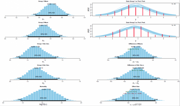
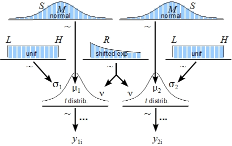
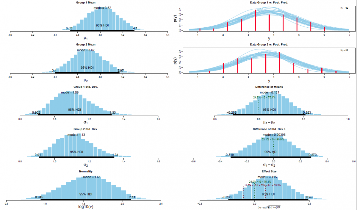
The posterior distribution is approximated by a powerful class of algorithms known as Markov chain Monte Carlo (MCMC) methods (named in analogy to the randomness of events observed at games in casinos). MCMC generates a large representative sample from the data which, in principle, allows to approximate the posterior distribution to an arbitrarily high degree of accuracy (as 𝑡→∞). The MCMC sample (or chain) contains a large number (i.e., > 1000) of combinations of the parameter values of interest. Our model of perceptual judgments contains the following parameters: < μ1, μ2, σ1, σ2, 𝜈 > (in all reported experiments). In other words, the MCMC algorithm randomly samples a very large n of combinations of θ from the posterior distribution. This representative sample of θ values is subsequently utilised in order to estimate various characteristics of the posterior (Gustafsson, Montelius, Starck, & Ljungberg, 2017), e.g., its mean, mode, median/medoid, standard deviation, etc. The thus obtained sample of parameter values can then be plotted in the form of a histogram in order to visualise the distributional properties and a prespecified high density interval (i.e., 95%) is then superimposed on the histogram in order to visualise the range of credible values for the parameter under investigation.
References
Plain numerical DOI: 10.1037/a0029146
DOI URL
directSciHub download
Show/hide publication abstract
Plain numerical DOI: 10.1111/j.2044-8317.2012.02063.x
DOI URL
directSciHub download
Show/hide publication abstract
Plain numerical DOI: 10.1177/1745691611406926
DOI URL
directSciHub download
Show/hide publication abstract
Plain numerical DOI: 10.1037/a0029146
DOI URL
directSciHub download
I just wanted to drop a quick note to say that I really enjoyed reading your article on Bayesian parameter estimation. It was informative and well-written, and I appreciated how you explained the benefits of this approach over NHST in a clear and concise manner.
I also found it helpful that you provided a link to the BEST.R function, and even mentioned that it has been ported to MATLAB and Python for those who prefer to use those programming languages.